1. 데이터 불러오기
# seaborn의 iris 데이터셋 로드
iris_df = pl.from_pandas(sns.load_dataset('iris'))
iris_df
# seaborn의 iris 데이터셋 로드
iris_df = pl.from_pandas(sns.load_dataset('iris'))
iris_df
2. 데이터 정보 확인
print("데이터 기본 정보:")
print(iris_df.glimpse())
print(iris_df.describe())
print("데이터 기본 정보:")
print(iris_df.glimpse())
print(iris_df.describe())
데이터 기본 정보:
Rows: 150
Columns: 5
$ sepal_length <f64> 5.1, 4.9, 4.7, 4.6, 5.0, 5.4, 4.6, 5.0, 4.4, 4.9
$ sepal_width  <f64> 3.5, 3.0, 3.2, 3.1, 3.6, 3.9, 3.4, 3.4, 2.9, 3.1
$ petal_length <f64> 1.4, 1.4, 1.3, 1.5, 1.4, 1.7, 1.4, 1.5, 1.4, 1.5
$ petal_width  <f64> 0.2, 0.2, 0.2, 0.2, 0.2, 0.4, 0.3, 0.2, 0.2, 0.1
$ species      <str> 'setosa', 'setosa', 'setosa', 'setosa', 'setosa', 'setosa', 'setosa', 'setosa', 'setosa', 'setosa'

None
shape: (9, 6)
┌────────────┬──────────────┬─────────────┬──────────────┬─────────────┬───────────┐
│ statistic  ┆ sepal_length ┆ sepal_width ┆ petal_length ┆ petal_width ┆ species   │
│ ---        ┆ ---          ┆ ---         ┆ ---          ┆ ---         ┆ ---       │
│ str        ┆ f64          ┆ f64         ┆ f64          ┆ f64         ┆ str       │
╞════════════╪══════════════╪═════════════╪══════════════╪═════════════╪═══════════╡
│ count      ┆ 150.0        ┆ 150.0       ┆ 150.0        ┆ 150.0       ┆ 150       │
│ null_count ┆ 0.0          ┆ 0.0         ┆ 0.0          ┆ 0.0         ┆ 0         │
│ mean       ┆ 5.843333     ┆ 3.057333    ┆ 3.758        ┆ 1.199333    ┆ null      │
│ std        ┆ 0.828066     ┆ 0.435866    ┆ 1.765298     ┆ 0.762238    ┆ null      │
│ min        ┆ 4.3          ┆ 2.0         ┆ 1.0          ┆ 0.1         ┆ setosa    │
│ 25%        ┆ 5.1          ┆ 2.8         ┆ 1.6          ┆ 0.3         ┆ null      │
│ 50%        ┆ 5.8          ┆ 3.0         ┆ 4.4          ┆ 1.3         ┆ null      │
│ 75%        ┆ 6.4          ┆ 3.3         ┆ 5.1          ┆ 1.8         ┆ null      │
│ max        ┆ 7.9          ┆ 4.4         ┆ 6.9          ┆ 2.5         ┆ virginica │
└────────────┴──────────────┴─────────────┴──────────────┴─────────────┴───────────┘
print(iris_df.shape)
print(iris_df.shape)
3. 데이터 전처리
3.1 결측값 확인
print("결측치 개수:")
print(iris_df.null_count())
print("결측치 개수:")
print(iris_df.null_count())
결측치 개수:
shape: (1, 5)
┌──────────────┬─────────────┬──────────────┬─────────────┬─────────┐
│ sepal_length ┆ sepal_width ┆ petal_length ┆ petal_width ┆ species │
│ ---          ┆ ---         ┆ ---          ┆ ---         ┆ ---     │
│ u32          ┆ u32         ┆ u32          ┆ u32         ┆ u32     │
╞══════════════╪═════════════╪══════════════╪═════════════╪═════════╡
│ 0            ┆ 0           ┆ 0            ┆ 0           ┆ 0       │
└──────────────┴─────────────┴──────────────┴─────────────┴─────────┘
4. 품종별 기술 통계
species_stats = (
    iris_df.group_by('species')
    .agg([
        pl.col('sepal_length').mean().alias('평균_꽃받침_길이'),
        pl.col('sepal_width').mean().alias('평균_꽃받침_너비'),
        pl.col('petal_length').mean().alias('평균_꽃잎_길이'),
        pl.col('petal_width').mean().alias('평균_꽃잎_너비'),
        pl.count().alias('샘플_수')
    ])
)
print("품종별 평균 측정값:")
print(species_stats)
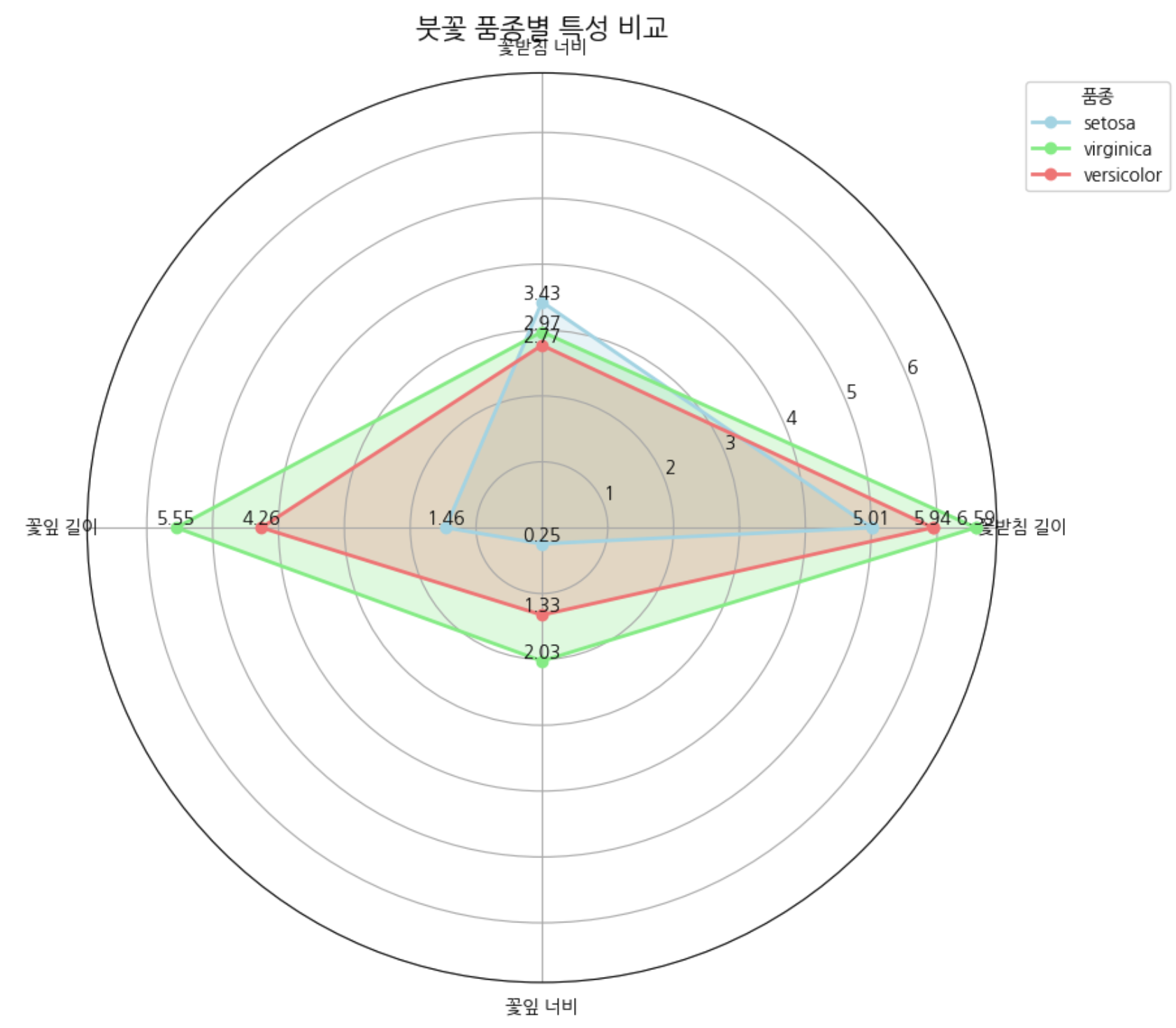
품종별 평균 측정값:
shape: (3, 6)
┌────────────┬──────────────────┬──────────────────┬────────────────┬────────────────┬─────────┐
│ species    ┆ 평균_꽃받침_길이 ┆ 평균_꽃받침_너비 ┆ 평균_꽃잎_길이 ┆ 평균_꽃잎_너비 ┆ 샘플_수 │
│ ---        ┆ ---              ┆ ---              ┆ ---            ┆ ---            ┆ ---     │
│ str        ┆ f64              ┆ f64              ┆ f64            ┆ f64            ┆ u32     │
╞════════════╪══════════════════╪══════════════════╪════════════════╪════════════════╪═════════╡
│ setosa     ┆ 5.006            ┆ 3.428            ┆ 1.462          ┆ 0.246          ┆ 50      │
│ virginica  ┆ 6.588            ┆ 2.974            ┆ 5.552          ┆ 2.026          ┆ 50      │
│ versicolor ┆ 5.936            ┆ 2.77             ┆ 4.26           ┆ 1.326          ┆ 50      │
└────────────┴──────────────────┴──────────────────┴────────────────┴────────────────┴─────────┘
# 그래프 크기 설정
plt.figure(figsize=(10, 8))

# 데이터 준비
categories = ['꽃받침 길이', '꽃받침 너비', '꽃잎 길이', '꽃잎 너비']
values = species_stats[['평균_꽃받침_길이', '평균_꽃받침_너비', '평균_꽃잎_길이', '평균_꽃잎_너비']].to_numpy()

# 각도 계산
angles = np.linspace(0, 2*np.pi, len(categories), endpoint=False)

# 닫힌 다각형을 위해 처음 값을 마지막에 추가
categories = np.concatenate((categories, [categories[0]]))
angles = np.concatenate((angles, [angles[0]]))
values = np.concatenate((values, values[:, [0]]), axis=1)

# 색상 설정
colors = ['lightblue', 'lightgreen', 'lightcoral']

# 레이더 차트 그리기
ax = plt.subplot(111, projection='polar')
for i, species in enumerate(species_stats['species']):
   ax.plot(angles, values[i], 'o-', linewidth=2, label=species, color=colors[i])
   ax.fill(angles, values[i], alpha=0.25, color=colors[i])

# 그래프 꾸미기
ax.set_xticks(angles[:-1])
ax.set_xticklabels(categories[:-1])
ax.set_title('붓꽃 품종별 특성 비교', pad=20, size=15)

# 데이터 레이블 추가
for i in range(len(species_stats)):
   for j in range(len(categories)-1):
       ax.text(angles[j], values[i,j], f'{values[i,j]:.2f}',
               ha='center', va='bottom')

plt.legend(title='품종', bbox_to_anchor=(1.2, 1))
plt.tight_layout()
plt.show()
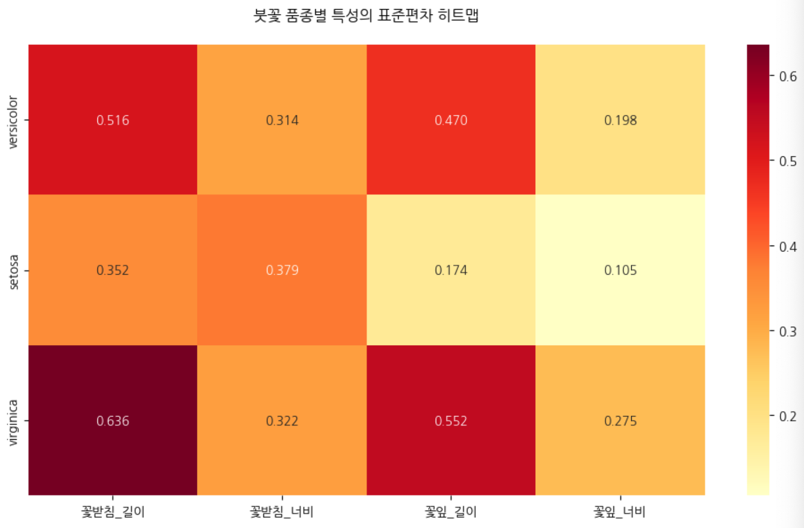
5. 특성별 분산 분석
variance_analysis = (
    iris_df.group_by('species')
    .agg([
        pl.col('sepal_length').std().alias('꽃받침_길이_표준편차'),
        pl.col('sepal_width').std().alias('꽃받침_너비_표준편차'),
        pl.col('petal_length').std().alias('꽃잎_길이_표준편차'),
        pl.col('petal_width').std().alias('꽃잎_너비_표준편차')
    ])
)
print("품종별 측정값 표준편차:")
print(variance_analysis)
품종별 측정값 표준편차:
shape: (3, 5)
┌────────────┬─────────────────────┬─────────────────────┬────────────────────┬────────────────────┐
│ species    ┆ 꽃받침_길이_표준편  ┆ 꽃받침_너비_표준편  ┆ 꽃잎_길이_표준편차 ┆ 꽃잎_너비_표준편차 │
│ ---        ┆ 차                  ┆ 차                  ┆ ---                ┆ ---                │
│ str        ┆ ---                 ┆ ---                 ┆ f64                ┆ f64                │
│            ┆ f64                 ┆ f64                 ┆                    ┆                    │
╞════════════╪═════════════════════╪═════════════════════╪════════════════════╪════════════════════╡
│ versicolor ┆ 0.516171            ┆ 0.313798            ┆ 0.469911           ┆ 0.197753           │
│ setosa     ┆ 0.35249             ┆ 0.379064            ┆ 0.173664           ┆ 0.105386           │
│ virginica  ┆ 0.63588             ┆ 0.322497            ┆ 0.551895           ┆ 0.27465            │
└────────────┴─────────────────────┴─────────────────────┴────────────────────┴────────────────────┘
plt.figure(figsize=(10, 6))

# 데이터 준비
features = ['꽃받침_길이_표준편차', '꽃받침_너비_표준편차',
           '꽃잎_길이_표준편차', '꽃잎_너비_표준편차']
data_matrix = variance_analysis[features].to_numpy()
species_labels = variance_analysis['species'].to_numpy()
feature_labels = [f.replace('_표준편차', '') for f in features]

# 히트맵 생성
sns.heatmap(data_matrix,
           annot=True,
           fmt='.3f',
           xticklabels=feature_labels,
           yticklabels=species_labels,
           cmap='YlOrRd')

plt.title('붓꽃 품종별 특성의 표준편차 히트맵', pad=20)
plt.tight_layout()
plt.show()
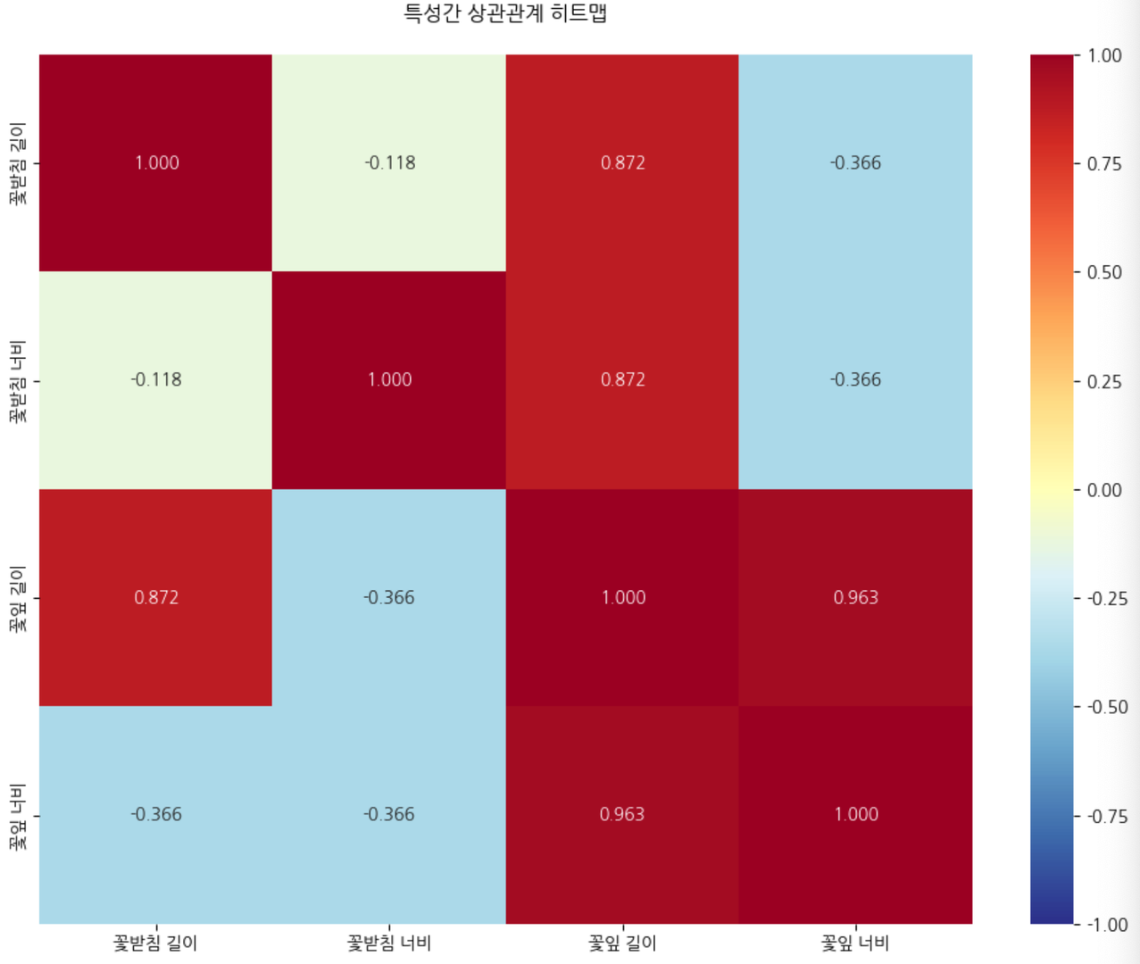
6. 특성간 상관관계
correlations = iris_df.select([
    pl.corr('sepal_length', 'sepal_width').alias('꽃받침_길이_너비_상관계수'),
    pl.corr('petal_length', 'petal_width').alias('꽃잎_길이_너비_상관계수'),
    pl.corr('sepal_length', 'petal_length').alias('꽃받침_꽃잎_길이_상관계수'),
    pl.corr('sepal_width', 'petal_width').alias('꽃받침_꽃잎_너비_상관계수')
])
print("특성간 상관관계:")
print(correlations)
특성간 상관관계:
shape: (1, 4)
┌────────────────────────┬────────────────────────┬────────────────────────┬───────────────────────┐
│ 꽃받침_길이_너비_상관  ┆ 꽃잎_길이_너비_상관계  ┆ 꽃받침_꽃잎_길이_상관  ┆ 꽃받침_꽃잎_너비_상관 │
│ 계수                   ┆ 수                     ┆ 계수                   ┆ 계수                  │
│ ---                    ┆ ---                    ┆ ---                    ┆ ---                   │
│ f64                    ┆ f64                    ┆ f64                    ┆ f64                   │
╞════════════════════════╪════════════════════════╪════════════════════════╪═══════════════════════╡
│ -0.11757               ┆ 0.962865               ┆ 0.871754               ┆ -0.366126             │
└────────────────────────┴────────────────────────┴────────────────────────┴───────────────────────┘
plt.figure(figsize=(10, 8))

# 상관계수 행렬 생성
features = ['꽃받침 길이', '꽃받침 너비', '꽃잎 길이', '꽃잎 너비']
corr_matrix = np.array([
    [1.0, correlations['꽃받침_길이_너비_상관계수'][0],
     correlations['꽃받침_꽃잎_길이_상관계수'][0],
     correlations['꽃받침_꽃잎_너비_상관계수'][0]],
    [correlations['꽃받침_길이_너비_상관계수'][0], 1.0,
     correlations['꽃받침_꽃잎_길이_상관계수'][0],
     correlations['꽃받침_꽃잎_너비_상관계수'][0]],
    [correlations['꽃받침_꽃잎_길이_상관계수'][0],
     correlations['꽃받침_꽃잎_너비_상관계수'][0], 1.0,
     correlations['꽃잎_길이_너비_상관계수'][0]],
    [correlations['꽃받침_꽃잎_너비_상관계수'][0],
     correlations['꽃받침_꽃잎_너비_상관계수'][0],
     correlations['꽃잎_길이_너비_상관계수'][0], 1.0]
])

# 히트맵 생성
sns.heatmap(corr_matrix,
            annot=True,
            fmt='.3f',
            cmap='RdYlBu_r',
            xticklabels=features,
            yticklabels=features,
            center=0,
            vmin=-1, vmax=1)

plt.title('특성간 상관관계 히트맵', pad=20)
plt.tight_layout()
plt.show()
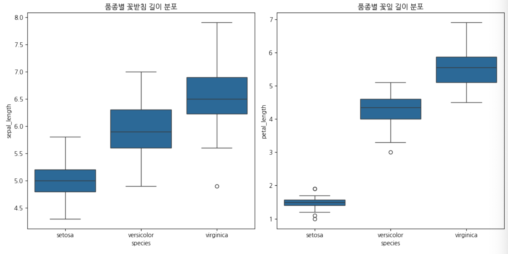
7. 품종별 사분위수 분석
quartile_analysis = (
    iris_df.group_by('species')
    .agg([
        pl.col('sepal_length').quantile(0.25).alias('꽃받침_길이_1사분위'),
        pl.col('sepal_length').quantile(0.75).alias('꽃받침_길이_3사분위'),
        pl.col('petal_length').quantile(0.25).alias('꽃잎_길이_1사분위'),
        pl.col('petal_length').quantile(0.75).alias('꽃잎_길이_3사분위')
    ])
)
print("품종별 사분위수 분석:")
print(quartile_analysis)
품종별 사분위수 분석:
shape: (3, 5)
┌────────────┬─────────────────────┬─────────────────────┬───────────────────┬───────────────────┐
│ species    ┆ 꽃받침_길이_1사분위 ┆ 꽃받침_길이_3사분위 ┆ 꽃잎_길이_1사분위 ┆ 꽃잎_길이_3사분위 │
│ ---        ┆ ---                 ┆ ---                 ┆ ---               ┆ ---               │
│ str        ┆ f64                 ┆ f64                 ┆ f64               ┆ f64               │
╞════════════╪═════════════════════╪═════════════════════╪═══════════════════╪═══════════════════╡
│ virginica  ┆ 6.2                 ┆ 6.9                 ┆ 5.1               ┆ 5.9               │
│ setosa     ┆ 4.8                 ┆ 5.2                 ┆ 1.4               ┆ 1.6               │
│ versicolor ┆ 5.6                 ┆ 6.3                 ┆ 4.0               ┆ 4.6               │
└────────────┴─────────────────────┴─────────────────────┴───────────────────┴───────────────────┘
plt.figure(figsize=(12, 6))
plt.subplot(1, 2, 1)
sns.boxplot(data=iris_df, x='species', y='sepal_length')
plt.title('품종별 꽃받침 길이 분포')

plt.subplot(1, 2, 2)
sns.boxplot(data=iris_df, x='species', y='petal_length')
plt.title('품종별 꽃잎 길이 분포')

plt.tight_layout()
plt.show()
plt.figure(figsize=(12, 6))
plt.subplot(1, 2, 1)
sns.boxplot(data=iris_df, x='species', y='sepal_length')
plt.title('품종별 꽃받침 길이 분포')

plt.subplot(1, 2, 2)
sns.boxplot(data=iris_df, x='species', y='petal_length')
plt.title('품종별 꽃잎 길이 분포')

plt.tight_layout()
plt.show()
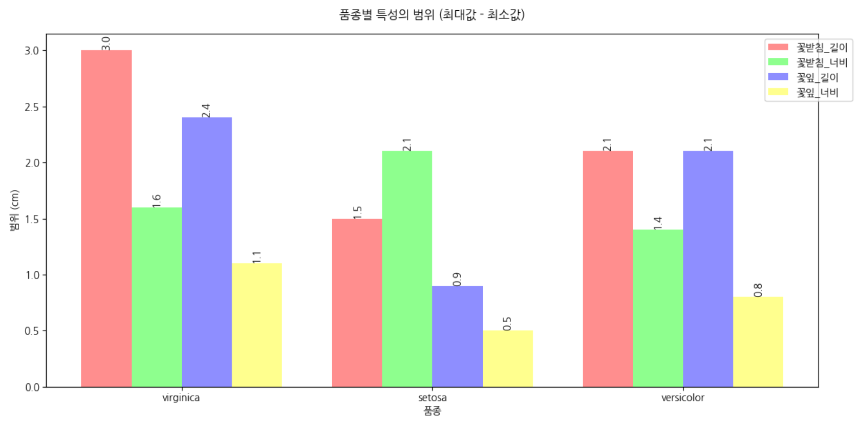
8. 특성별 범위 분석
range_analysis = (
    iris_df.group_by('species')
    .agg([
        (pl.col('sepal_length').max() - pl.col('sepal_length').min()).alias('꽃받침_길이_범위'),
        (pl.col('sepal_width').max() - pl.col('sepal_width').min()).alias('꽃받침_너비_범위'),
        (pl.col('petal_length').max() - pl.col('petal_length').min()).alias('꽃잎_길이_범위'),
        (pl.col('petal_width').max() - pl.col('petal_width').min()).alias('꽃잎_너비_범위')
    ])
)
print("품종별 측정값 범위:")
print(range_analysis)
품종별 측정값 범위:
shape: (3, 5)
┌────────────┬──────────────────┬──────────────────┬────────────────┬────────────────┐
│ species    ┆ 꽃받침_길이_범위 ┆ 꽃받침_너비_범위 ┆ 꽃잎_길이_범위 ┆ 꽃잎_너비_범위 │
│ ---        ┆ ---              ┆ ---              ┆ ---            ┆ ---            │
│ str        ┆ f64              ┆ f64              ┆ f64            ┆ f64            │
╞════════════╪══════════════════╪══════════════════╪════════════════╪════════════════╡
│ virginica  ┆ 3.0              ┆ 1.6              ┆ 2.4            ┆ 1.1            │
│ setosa     ┆ 1.5              ┆ 2.1              ┆ 0.9            ┆ 0.5            │
│ versicolor ┆ 2.1              ┆ 1.4              ┆ 2.1            ┆ 0.8            │
└────────────┴──────────────────┴──────────────────┴────────────────┴────────────────┘
plt.figure(figsize=(12, 6))

# 데이터 준비
features = ['꽃받침_길이_범위', '꽃받침_너비_범위', '꽃잎_길이_범위', '꽃잎_너비_범위']
x = np.arange(len(range_analysis))
width = 0.2

# 각 특성별 막대 그래프
colors = ['#FF9999', '#99FF99', '#9999FF', '#FFFF99']
for i, feature in enumerate(features):
    plt.bar(x + i*width,
            range_analysis[feature],
            width,
            label=feature.replace('_범위', ''),
            color=colors[i])

# 그래프 꾸미기
plt.title('품종별 특성의 범위 (최대값 - 최소값)', pad=15)
plt.xlabel('품종')
plt.ylabel('범위 (cm)')
plt.xticks(x + width*1.5, range_analysis['species'])
plt.legend(bbox_to_anchor=(1.05, 1))

# 값 레이블 추가
for i, feature in enumerate(features):
    for j, v in enumerate(range_analysis[feature]):
        plt.text(x[j] + i*width, v, f'{v:.1f}',
                ha='center', va='bottom', rotation=90)

plt.tight_layout()
plt.show()
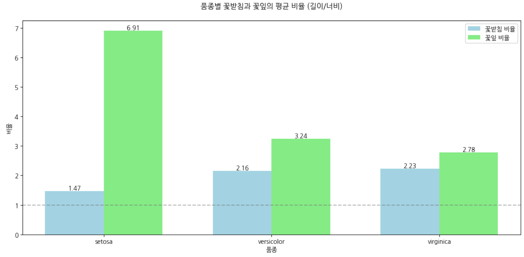
9. 비율 분석 (꽃받침 길이/너비, 꽃잎 길이/너비)
ratio_analysis = (
    iris_df.with_columns([
        (pl.col('sepal_length') / pl.col('sepal_width')).alias('꽃받침_비율'),
        (pl.col('petal_length') / pl.col('petal_width')).alias('꽃잎_비율')
    ])
    .group_by('species')
    .agg([
        pl.col('꽃받침_비율').mean().alias('평균_꽃받침_비율'),
        pl.col('꽃잎_비율').mean().alias('평균_꽃잎_비율')
    ])
)
print("품종별 비율 분석:")
print(ratio_analysis)
품종별 비율 분석:
shape: (3, 3)
┌────────────┬──────────────────┬────────────────┐
│ species    ┆ 평균_꽃받침_비율 ┆ 평균_꽃잎_비율 │
│ ---        ┆ ---              ┆ ---            │
│ str        ┆ f64              ┆ f64            │
╞════════════╪══════════════════╪════════════════╡
│ setosa     ┆ 1.470188         ┆ 6.908          │
│ versicolor ┆ 2.160402         ┆ 3.242837       │
│ virginica  ┆ 2.230453         ┆ 2.780662       │
└────────────┴──────────────────┴────────────────┘
# 그래프 크기 설정
plt.figure(figsize=(12, 6))

# 데이터 준비
x = np.arange(len(ratio_analysis))
width = 0.35

# numpy 배열로 변환
sepal_ratios = ratio_analysis['평균_꽃받침_비율'].to_numpy()
petal_ratios = ratio_analysis['평균_꽃잎_비율'].to_numpy()

# 막대 그래프 생성
plt.bar(x - width/2, sepal_ratios,
        width, label='꽃받침 비율', color='lightblue')
plt.bar(x + width/2, petal_ratios,
        width, label='꽃잎 비율', color='lightgreen')

# 그래프 꾸미기
plt.title('품종별 꽃받침과 꽃잎의 평균 비율 (길이/너비)', pad=20)
plt.xlabel('품종')
plt.ylabel('비율')
plt.xticks(x, ratio_analysis['species'])
plt.legend()

# 데이터 레이블 추가
for i in x:
    # 꽃받침 비율
    plt.text(i - width/2, sepal_ratios[i],
             f'{sepal_ratios[i]:.2f}',
             ha='center', va='bottom')
    # 꽃잎 비율
    plt.text(i + width/2, petal_ratios[i],
             f'{petal_ratios[i]:.2f}',
             ha='center', va='bottom')

# 수평 기준선 추가 (비율 1:1)
plt.axhline(y=1, color='gray', linestyle='--', alpha=0.5)

plt.tight_layout()
plt.show()
10. 종합 통계
summary_stats = {
    '전체_샘플수': iris_df.shape[0],
    '품종별_샘플수': iris_df.group_by('species').count(),
    '전체_꽃받침_길이_평균': round(iris_df['sepal_length'].mean(),2),
    '전체_꽃잎_길이_평균': round(iris_df['petal_length'].mean(),2),
    '가장_긴_꽃받침': iris_df['sepal_length'].max(),
    '가장_긴_꽃잎': iris_df['petal_length'].max()
}
print("종합 통계:")
print(summary_stats)
종합 통계:
{'전체_샘플수': 150, '품종별_샘플수': shape: (3, 2)
┌────────────┬───────┐
│ species    ┆ count │
│ ---        ┆ ---   │
│ str        ┆ u32   │
╞════════════╪═══════╡
│ versicolor ┆ 50    │
│ setosa     ┆ 50    │
│ virginica  ┆ 50    │
└────────────┴───────┘, '전체_꽃받침_길이_평균': 5.84, '전체_꽃잎_길이_평균': 3.76, '가장_긴_꽃받침': 7.9, '가장_긴_꽃잎': 6.9}
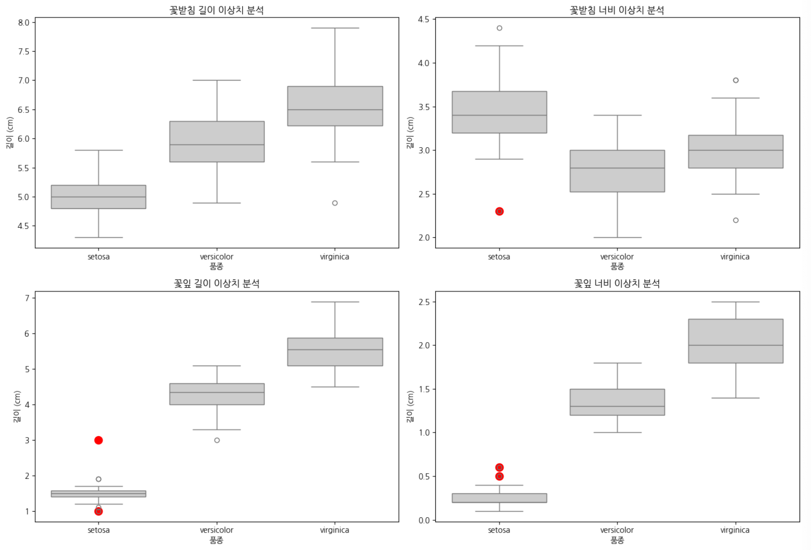
11. 이상치 분석
def find_outliers(df, column):
    Q1 = df[column].quantile(0.25)
    Q3 = df[column].quantile(0.75)
    IQR = Q3 - Q1
    lower_bound = Q1 - 1.5 * IQR
    upper_bound = Q3 + 1.5 * IQR
    return df.filter(
        (pl.col(column) < lower_bound) | (pl.col(column) > upper_bound)
    )

outliers = {}
for column in ['sepal_length', 'sepal_width', 'petal_length', 'petal_width']:
    outliers[column] = iris_df.group_by('species').map_groups(
        lambda group: find_outliers(group, column)
    )

print("이상치 분석:")
for column, outlier_data in outliers.items():
    print(f"\n{column} 이상치:")
    print(outlier_data)
이상치 분석:

sepal_length 이상치:
shape: (1, 5)
┌──────────────┬─────────────┬──────────────┬─────────────┬───────────┐
│ sepal_length ┆ sepal_width ┆ petal_length ┆ petal_width ┆ species   │
│ ---          ┆ ---         ┆ ---          ┆ ---         ┆ ---       │
│ f64          ┆ f64         ┆ f64          ┆ f64         ┆ str       │
╞══════════════╪═════════════╪══════════════╪═════════════╪═══════════╡
│ 4.9          ┆ 2.5         ┆ 4.5          ┆ 1.7         ┆ virginica │
└──────────────┴─────────────┴──────────────┴─────────────┴───────────┘

sepal_width 이상치:
shape: (1, 5)
┌──────────────┬─────────────┬──────────────┬─────────────┬─────────┐
│ sepal_length ┆ sepal_width ┆ petal_length ┆ petal_width ┆ species │
│ ---          ┆ ---         ┆ ---          ┆ ---         ┆ ---     │
│ f64          ┆ f64         ┆ f64          ┆ f64         ┆ str     │
╞══════════════╪═════════════╪══════════════╪═════════════╪═════════╡
│ 4.5          ┆ 2.3         ┆ 1.3          ┆ 0.3         ┆ setosa  │
└──────────────┴─────────────┴──────────────┴─────────────┴─────────┘

petal_length 이상치:
shape: (2, 5)
┌──────────────┬─────────────┬──────────────┬─────────────┬────────────┐
│ sepal_length ┆ sepal_width ┆ petal_length ┆ petal_width ┆ species    │
│ ---          ┆ ---         ┆ ---          ┆ ---         ┆ ---        │
│ f64          ┆ f64         ┆ f64          ┆ f64         ┆ str        │
╞══════════════╪═════════════╪══════════════╪═════════════╪════════════╡
│ 4.6          ┆ 3.6         ┆ 1.0          ┆ 0.2         ┆ setosa     │
│ 5.1          ┆ 2.5         ┆ 3.0          ┆ 1.1         ┆ versicolor │
└──────────────┴─────────────┴──────────────┴─────────────┴────────────┘

petal_width 이상치:
shape: (2, 5)
┌──────────────┬─────────────┬──────────────┬─────────────┬─────────┐
│ sepal_length ┆ sepal_width ┆ petal_length ┆ petal_width ┆ species │
│ ---          ┆ ---         ┆ ---          ┆ ---         ┆ ---     │
│ f64          ┆ f64         ┆ f64          ┆ f64         ┆ str     │
╞══════════════╪═════════════╪══════════════╪═════════════╪═════════╡
│ 5.1          ┆ 3.3         ┆ 1.7          ┆ 0.5         ┆ setosa  │
│ 5.0          ┆ 3.5         ┆ 1.6          ┆ 0.6         ┆ setosa  │
└──────────────┴─────────────┴──────────────┴─────────────┴─────────┘
# 그래프 크기 설정
plt.figure(figsize=(15, 10))

# 특성 목록
features = ['sepal_length', 'sepal_width', 'petal_length', 'petal_width']
titles = ['꽃받침 길이', '꽃받침 너비', '꽃잎 길이', '꽃잎 너비']

# 2x2 서브플롯 생성
for idx, (feature, title) in enumerate(zip(features, titles), 1):
    plt.subplot(2, 2, idx)

    # 박스플롯 그리기
    sns.boxplot(data=iris_df, x='species', y=feature, color='lightgray')

    # 이상치 표시
    if feature in outliers and len(outliers[feature]) > 0:
        outlier_data = outliers[feature]
        for species in iris_df['species'].unique():
            species_outliers = outlier_data.filter(pl.col('species') == species)
            if len(species_outliers) > 0:
                x = list(iris_df['species'].unique()).index(species)
                plt.scatter([x] * len(species_outliers),
                          species_outliers[feature],
                          color='red',
                          s=100,
                          label='이상치' if idx == 1 else None)

    plt.title(f'{title} 이상치 분석')
    plt.xlabel('품종')
    plt.ylabel('길이 (cm)')

# 범례 추가 (첫 번째 서브플롯에만)
if any(len(outliers[f]) > 0 for f in features):
    plt.legend(bbox_to_anchor=(1.05, 1), loc='upper left')

plt.tight_layout()
plt.show()