DataFrame(데이터프레임)
1. DataFrame (데이터프레임) 이란?
데이터프레임(DataFrame)은 시리즈를 기반으로 여러 개의 행(Row)과 열(Column)로 이루어진 2차원 데이터 배열 구조입니다. 엑셀 스프레드시트와 유사한 테이블(표) 형태로 이루어져 있어 데이터를 다루기에 적합한 자료구조입니다.
DataFrame은 여러 개의 행(Row)과 열(Column)로 구성됩니다.
- 단일 열은 하나의 데이터 타입만 가질 수 있으며, 시리즈로 반환됩니다.
- 각 행에는 리스트와 같이 다양한 데이터 유형을 포함할 수 있습니다.
2. DataFrame 생성
pl.DataFrame(데이터) 를 사용하여 DataFrame을 생성할 수 있습니다. 데이터에는 딕셔너리, numpy 배열, 시리즈 데이터 형태가 들어갈 수 있습니다.
2.1 Dictionary로 생성하기
from datetime import datetime
import polars as pl

data = {
    "integer": [1, 2, 3, 4, 5],
    "date": [
        datetime(2022, 1, 1),
        datetime(2022, 1, 2),
        datetime(2022, 1, 3),
        datetime(2022, 1, 4),
        datetime(2022, 1, 5),
    ],
    "float": [4.0, 5.0, 6.0, 7.0, 8.0],
    "string": ["a", "b", "c", "d", "e"],
}

# 데이터프레임 생성하기
df = pl.DataFrame(data)
print(df)
from datetime import datetime
import polars as pl
data = {
"integer": [1, 2, 3, 4, 5],
"date": [
datetime(2022, 1, 1),
datetime(2022, 1, 2),
datetime(2022, 1, 3),
datetime(2022, 1, 4),
datetime(2022, 1, 5),
],
"float": [4.0, 5.0, 6.0, 7.0, 8.0],
"string": ["a", "b", "c", "d", "e"],
}
# 데이터프레임 생성하기
df = pl.DataFrame(data)
print(df)shape: (5, 4)
┌─────────┬─────────────────────┬───────┬────────┐
│ integer ┆ date ┆ float ┆ string │
│ --- ┆ --- ┆ --- ┆ --- │
│ i64 ┆ datetime[μs] ┆ f64 ┆ str │
╞═════════╪═════════════════════╪═══════╪════════╡
│ 1 ┆ 2022-01-01 00:00:00 ┆ 4.0 ┆ a │
│ 2 ┆ 2022-01-02 00:00:00 ┆ 5.0 ┆ b │
│ 3 ┆ 2022-01-03 00:00:00 ┆ 6.0 ┆ c │
│ 4 ┆ 2022-01-04 00:00:00 ┆ 7.0 ┆ d │
│ 5 ┆ 2022-01-05 00:00:00 ┆ 8.0 ┆ e │
└─────────┴─────────────────────┴───────┴────────┘shape: (5, 4)
┌─────────┬─────────────────────┬───────┬────────┐
│ integer ┆ date ┆ float ┆ string │
│ --- ┆ --- ┆ --- ┆ --- │
│ i64 ┆ datetime[μs] ┆ f64 ┆ str │
╞═════════╪═════════════════════╪═══════╪════════╡
│ 1 ┆ 2022-01-01 00:00:00 ┆ 4.0 ┆ a │
│ 2 ┆ 2022-01-02 00:00:00 ┆ 5.0 ┆ b │
│ 3 ┆ 2022-01-03 00:00:00 ┆ 6.0 ┆ c │
│ 4 ┆ 2022-01-04 00:00:00 ┆ 7.0 ┆ d │
│ 5 ┆ 2022-01-05 00:00:00 ┆ 8.0 ┆ e │
└─────────┴─────────────────────┴───────┴────────┘2.2 Series 리스트로 생성하기
data = [
    pl.Series("col1", [1, 2], dtype=pl.Float32),
    pl.Series("col2", [3, 4], dtype=pl.Int64),
]
df2 = pl.DataFrame(data)
print(df2)
data = [
pl.Series("col1", [1, 2], dtype=pl.Float32),
pl.Series("col2", [3, 4], dtype=pl.Int64),
]
df2 = pl.DataFrame(data)
print(df2)shape: (2, 2)
┌──────┬──────┐
│ col1 ┆ col2 │
│ --- ┆ --- │
│ f32 ┆ i64 │
╞══════╪══════╡
│ 1.0 ┆ 3 │
│ 2.0 ┆ 4 │
└──────┴──────┘shape: (2, 2)
┌──────┬──────┐
│ col1 ┆ col2 │
│ --- ┆ --- │
│ f32 ┆ i64 │
╞══════╪══════╡
│ 1.0 ┆ 3 │
│ 2.0 ┆ 4 │
└──────┴──────┘2.3 중첩 리스트로 생성하기
중첩리스트 형태로 데이터를 생성하고 schema 매개변수를 사용하여 열 이름 지정합니다.
data = [[1, 2, 3], [4, 5, 6]]
df3 = pl.DataFrame(data, schema=["a", "b", "c"])
print(df3)
data = [[1, 2, 3], [4, 5, 6]]
df3 = pl.DataFrame(data, schema=["a", "b", "c"])
print(df3)shape: (2, 3)
┌─────┬─────┬─────┐
│ a ┆ b ┆ c │
│ --- ┆ --- ┆ --- │
│ i64 ┆ i64 ┆ i64 │
╞═════╪═════╪═════╡
│ 1 ┆ 2 ┆ 3 │
│ 4 ┆ 5 ┆ 6 │
└─────┴─────┴─────┘shape: (2, 3)
┌─────┬─────┬─────┐
│ a ┆ b ┆ c │
│ --- ┆ --- ┆ --- │
│ i64 ┆ i64 ┆ i64 │
╞═════╪═════╪═════╡
│ 1 ┆ 2 ┆ 3 │
│ 4 ┆ 5 ┆ 6 │
└─────┴─────┴─────┘중첩 리스트로 데이터 프레임을 생성할 경우 행을 먼저 채우고 열을 채우게 됩니다. 만약, 열을 기준으로 먼저 채우고 싶으시다면 orient="col" 속성을 주시면 됩니다.
import numpy as np

data = np.array([(1, 2), (3, 4)], dtype=np.int64)
df6 = pl.DataFrame(data, schema=["a", "b"], orient="col")
print(df6)
import numpy as np
data = np.array([(1, 2), (3, 4)], dtype=np.int64)
df6 = pl.DataFrame(data, schema=["a", "b"], orient="col")
print(df6)- orient
- col : 열을 기준으로 데이터를 넣습니다.
- row(기본값) : 행을 기준으로 데이터를 넣습니다.
shape: (2, 2)
┌─────┬─────┐
│ a   ┆ b   │
│ --- ┆ --- │
│ i64 ┆ i64 │
╞═════╪═════╡
│ 1   ┆ 3   │
│ 2   ┆ 4   │
└─────┴─────┘
shape: (2, 2)
┌─────┬─────┐
│ a ┆ b │
│ --- ┆ --- │
│ i64 ┆ i64 │
╞═════╪═════╡
│ 1 ┆ 3 │
│ 2 ┆ 4 │
└─────┴─────┘3. 데이터 타입
3.1 dtypes
데이터 타입은 데이터프레임을 출력할 때 헤더에서 확인할 수 있습니다. dtypes으로 데이터프레임 안에 있는 열의 데이터 타입(자료형)을 차례대로 확인할 수 있습니다.
print(df.dtypes)print(df.dtypes)[Int64, Datetime(time_unit='us', time_zone=None), Float64, String][Int64, Datetime(time_unit='us', time_zone=None), Float64, String]3.2 schema
schema는 컬럼명과 데이터 타입을 같이 확인할 수 있으며, (컬럼명, 데이터 타입) 순서대로 튜플 형태로 출력됩니다.
print(df.schema)print(df.schema)Schema([('integer', Int64), ('date', Datetime(time_unit='us', time_zone=None)), ('float', Float64), ('string', String)])Schema([('integer', Int64), ('date', Datetime(time_unit='us', time_zone=None)), ('float', Float64), ('string', String)])데이터프레임 생성 시에 schema 매개변수를 사용하여 열의 타입을 지정할 수도 있습니다.
-
{name
}의 딕셔너리 형태 data = {"col1": [0, 2], "col2": [3, 7]} df4 = pl.DataFrame(data, schema={"col1": pl.Float32, "col2": pl.Int64}) print(df4)data = {"col1": [0, 2], "col2": [3, 7]} df4 = pl.DataFrame(data, schema={"col1": pl.Float32, "col2": pl.Int64}) print(df4)shape: (2, 2) ┌──────┬──────┐ │ col1 ┆ col2 │ │ --- ┆ --- │ │ f32 ┆ i64 │ ╞══════╪══════╡ │ 0.0 ┆ 3 │ │ 2.0 ┆ 7 │ └──────┴──────┘shape: (2, 2) ┌──────┬──────┐ │ col1 ┆ col2 │ │ --- ┆ --- │ │ f32 ┆ i64 │ ╞══════╪══════╡ │ 0.0 ┆ 3 │ │ 2.0 ┆ 7 │ └──────┴──────┘ -
(name
) 리스트 형태 df5 = pl.DataFrame(data, schema=[("col1", pl.Float32), ("col2", pl.Int64)]) print(df5)df5 = pl.DataFrame(data, schema=[("col1", pl.Float32), ("col2", pl.Int64)]) print(df5)shape: (2, 2) ┌──────┬──────┐ │ col1 ┆ col2 │ │ --- ┆ --- │ │ f32 ┆ i64 │ ╞══════╪══════╡ │ 0.0 ┆ 3 │ │ 2.0 ┆ 7 │ └──────┴──────┘shape: (2, 2) ┌──────┬──────┐ │ col1 ┆ col2 │ │ --- ┆ --- │ │ f32 ┆ i64 │ ╞══════╪══════╡ │ 0.0 ┆ 3 │ │ 2.0 ┆ 7 │ └──────┴──────┘
schema를 사용하여 생성하실 때,
- 스키마에 제공된 컬럼명 수는 데이터 차원 수와 일치해야 합니다.
- 데이터 타입을 따로 지정하지 않거나 기본값인 None으로 설정한 컬럼들은 자동으로 타입을 설정합니다.
- 기본 데이터의 컬럼명과 일치하지 않는 열 이름 목록을 제공하면 제공된 컬럼명이 해당 목록을 덮어씁니다.
3.3 cast
딕셔너리 형태로 {컬럼명 : 데이터 타입} 주어 열을 지정된 데이터 타입으로 형변환합니다.
# df.cast({"컬럼명": 데이터타입})
print(df.cast({"integer": pl.Float32, "float": pl.UInt8}))
# df.cast({"컬럼명": 데이터타입})
print(df.cast({"integer": pl.Float32, "float": pl.UInt8}))shape: (5, 4)
┌─────────┬─────────────────────┬───────┬────────┐
│ integer ┆ date ┆ float ┆ string │
│ --- ┆ --- ┆ --- ┆ --- │
│ f32 ┆ datetime[μs] ┆ i32 ┆ str │
╞═════════╪═════════════════════╪═══════╪════════╡
│ 1.0 ┆ 2022-01-01 00:00:00 ┆ 4 ┆ a │
│ 2.0 ┆ 2022-01-02 00:00:00 ┆ 5 ┆ b │
│ 3.0 ┆ 2022-01-03 00:00:00 ┆ 6 ┆ c │
│ 4.0 ┆ 2022-01-04 00:00:00 ┆ 7 ┆ d │
│ 5.0 ┆ 2022-01-05 00:00:00 ┆ 8 ┆ e │
└─────────┴─────────────────────┴───────┴────────┘shape: (5, 4)
┌─────────┬─────────────────────┬───────┬────────┐
│ integer ┆ date ┆ float ┆ string │
│ --- ┆ --- ┆ --- ┆ --- │
│ f32 ┆ datetime[μs] ┆ i32 ┆ str │
╞═════════╪═════════════════════╪═══════╪════════╡
│ 1.0 ┆ 2022-01-01 00:00:00 ┆ 4 ┆ a │
│ 2.0 ┆ 2022-01-02 00:00:00 ┆ 5 ┆ b │
│ 3.0 ┆ 2022-01-03 00:00:00 ┆ 6 ┆ c │
│ 4.0 ┆ 2022-01-04 00:00:00 ┆ 7 ┆ d │
│ 5.0 ┆ 2022-01-05 00:00:00 ┆ 8 ┆ e │
└─────────┴─────────────────────┴───────┴────────┘selectors로 모든 열을 한 번에 같은 데이터 타입으로 변환할 수도 있습니다.
import polars.selectors as cs
print(df.cast({cs.numeric(): pl.UInt32, cs.temporal(): pl.String}))
import polars.selectors as cs
print(df.cast({cs.numeric(): pl.UInt32, cs.temporal(): pl.String}))shape: (5, 4)
┌─────────┬────────────────────────────┬───────┬────────┐
│ integer ┆ date ┆ float ┆ string │
│ --- ┆ --- ┆ --- ┆ --- │
│ u32 ┆ str ┆ u32 ┆ str │
╞═════════╪════════════════════════════╪═══════╪════════╡
│ 1 ┆ 2022-01-01 00:00:00.000000 ┆ 4 ┆ a │
│ 2 ┆ 2022-01-02 00:00:00.000000 ┆ 5 ┆ b │
│ 3 ┆ 2022-01-03 00:00:00.000000 ┆ 6 ┆ c │
│ 4 ┆ 2022-01-04 00:00:00.000000 ┆ 7 ┆ d │
│ 5 ┆ 2022-01-05 00:00:00.000000 ┆ 8 ┆ e │
└─────────┴────────────────────────────┴───────┴────────┘shape: (5, 4)
┌─────────┬────────────────────────────┬───────┬────────┐
│ integer ┆ date ┆ float ┆ string │
│ --- ┆ --- ┆ --- ┆ --- │
│ u32 ┆ str ┆ u32 ┆ str │
╞═════════╪════════════════════════════╪═══════╪════════╡
│ 1 ┆ 2022-01-01 00:00:00.000000 ┆ 4 ┆ a │
│ 2 ┆ 2022-01-02 00:00:00.000000 ┆ 5 ┆ b │
│ 3 ┆ 2022-01-03 00:00:00.000000 ┆ 6 ┆ c │
│ 4 ┆ 2022-01-04 00:00:00.000000 ┆ 7 ┆ d │
│ 5 ┆ 2022-01-05 00:00:00.000000 ┆ 8 ┆ e │
└─────────┴────────────────────────────┴───────┴────────┘모든 열을 단일 데이터 타입으로 변환할 수 있습니다.
print(df.cast(pl.String))print(df.cast(pl.String))shape: (5, 4)
┌─────────┬────────────────────────────┬───────┬────────┐
│ integer ┆ date ┆ float ┆ string │
│ --- ┆ --- ┆ --- ┆ --- │
│ str ┆ str ┆ str ┆ str │
╞═════════╪════════════════════════════╪═══════╪════════╡
│ 1 ┆ 2022-01-01 00:00:00.000000 ┆ 4.0 ┆ a │
│ 2 ┆ 2022-01-02 00:00:00.000000 ┆ 5.0 ┆ b │
│ 3 ┆ 2022-01-03 00:00:00.000000 ┆ 6.0 ┆ c │
│ 4 ┆ 2022-01-04 00:00:00.000000 ┆ 7.0 ┆ d │
│ 5 ┆ 2022-01-05 00:00:00.000000 ┆ 8.0 ┆ e │
└─────────┴────────────────────────────┴───────┴────────┘shape: (5, 4)
┌─────────┬────────────────────────────┬───────┬────────┐
│ integer ┆ date ┆ float ┆ string │
│ --- ┆ --- ┆ --- ┆ --- │
│ str ┆ str ┆ str ┆ str │
╞═════════╪════════════════════════════╪═══════╪════════╡
│ 1 ┆ 2022-01-01 00:00:00.000000 ┆ 4.0 ┆ a │
│ 2 ┆ 2022-01-02 00:00:00.000000 ┆ 5.0 ┆ b │
│ 3 ┆ 2022-01-03 00:00:00.000000 ┆ 6.0 ┆ c │
│ 4 ┆ 2022-01-04 00:00:00.000000 ┆ 7.0 ┆ d │
│ 5 ┆ 2022-01-05 00:00:00.000000 ┆ 8.0 ┆ e │
└─────────┴────────────────────────────┴───────┴────────┘데이터 타입과 일치하는 모든 열을 다른 데이터 타입으로 변환할 수도 있습니다.
print(df.cast({pl.Datetime: pl.Date}))print(df.cast({pl.Datetime: pl.Date}))shape: (5, 4)
┌─────────┬────────────┬───────┬────────┐
│ integer ┆ date ┆ float ┆ string │
│ --- ┆ --- ┆ --- ┆ --- │
│ i64 ┆ date ┆ f64 ┆ str │
╞═════════╪════════════╪═══════╪════════╡
│ 1 ┆ 2022-01-01 ┆ 4.0 ┆ a │
│ 2 ┆ 2022-01-02 ┆ 5.0 ┆ b │
│ 3 ┆ 2022-01-03 ┆ 6.0 ┆ c │
│ 4 ┆ 2022-01-04 ┆ 7.0 ┆ d │
│ 5 ┆ 2022-01-05 ┆ 8.0 ┆ e │
└─────────┴────────────┴───────┴────────┘shape: (5, 4)
┌─────────┬────────────┬───────┬────────┐
│ integer ┆ date ┆ float ┆ string │
│ --- ┆ --- ┆ --- ┆ --- │
│ i64 ┆ date ┆ f64 ┆ str │
╞═════════╪════════════╪═══════╪════════╡
│ 1 ┆ 2022-01-01 ┆ 4.0 ┆ a │
│ 2 ┆ 2022-01-02 ┆ 5.0 ┆ b │
│ 3 ┆ 2022-01-03 ┆ 6.0 ┆ c │
│ 4 ┆ 2022-01-04 ┆ 7.0 ┆ d │
│ 5 ┆ 2022-01-05 ┆ 8.0 ┆ e │
└─────────┴────────────┴───────┴────────┘strict 매개변수를 True(기본값)로 설정하면, 형변환을 수행할 수 없는 경우 오류를 출력합니다.
print(df.cast({pl.String: pl.Datetime}, strict=True))print(df.cast({pl.String: pl.Datetime}, strict=True))InvalidOperationError: conversion from `str` to `datetime[μs]` failed in column 'string' for 5 out of 5 values: ["a", "b", … "e"]
You might want to try:
- setting `strict=False` to set values that cannot be converted to `null`
- using `str.strptime`, `str.to_date`, or `str.to_datetime` and providing a format stringInvalidOperationError: conversion from `str` to `datetime[μs]` failed in column 'string' for 5 out of 5 values: ["a", "b", … "e"]
You might want to try:
- setting `strict=False` to set values that cannot be converted to `null`
- using `str.strptime`, `str.to_date`, or `str.to_datetime` and providing a format string만약, False로 설정할 경우, 오류가 나는 열의 값은 null로 반환됩니다.
print(df.cast({pl.String: pl.Datetime}, strict=False))print(df.cast({pl.String: pl.Datetime}, strict=False))shape: (5, 4)
┌─────────┬─────────────────────┬───────┬──────────────┐
│ integer ┆ date ┆ float ┆ string │
│ --- ┆ --- ┆ --- ┆ --- │
│ i64 ┆ datetime[μs] ┆ f64 ┆ datetime[μs] │
╞═════════╪═════════════════════╪═══════╪══════════════╡
│ 1 ┆ 2022-01-01 00:00:00 ┆ 4.0 ┆ null │
│ 2 ┆ 2022-01-02 00:00:00 ┆ 5.0 ┆ null │
│ 3 ┆ 2022-01-03 00:00:00 ┆ 6.0 ┆ null │
│ 4 ┆ 2022-01-04 00:00:00 ┆ 7.0 ┆ null │
│ 5 ┆ 2022-01-05 00:00:00 ┆ 8.0 ┆ null │
└─────────┴─────────────────────┴───────┴──────────────┘shape: (5, 4)
┌─────────┬─────────────────────┬───────┬──────────────┐
│ integer ┆ date ┆ float ┆ string │
│ --- ┆ --- ┆ --- ┆ --- │
│ i64 ┆ datetime[μs] ┆ f64 ┆ datetime[μs] │
╞═════════╪═════════════════════╪═══════╪══════════════╡
│ 1 ┆ 2022-01-01 00:00:00 ┆ 4.0 ┆ null │
│ 2 ┆ 2022-01-02 00:00:00 ┆ 5.0 ┆ null │
│ 3 ┆ 2022-01-03 00:00:00 ┆ 6.0 ┆ null │
│ 4 ┆ 2022-01-04 00:00:00 ┆ 7.0 ┆ null │
│ 5 ┆ 2022-01-05 00:00:00 ┆ 8.0 ┆ null │
└─────────┴─────────────────────┴───────┴──────────────┘4. 데이터 사전 분석
데이터프레임의 기본 정보를 간단히 살펴보도록 하겠습니다.
4.1 사전 분석에 사용할 함수
- glimpse(): DataFrame을 구성하는 행과 열에 대한 정보를 나타내 주는 함수
- head(n), limit(n) : DataFrame의 처음부터 n개의 행을 출력
- tail(n): DataFrame의 마지막 n개의 행을 출력
- describe(): Series, DataFrame의 각 열에 대한 요약 통계
- shape: DataFrame의 크기(행/열 개수) 확인
- height: DataFrame의 행 개수 확인
- width: DataFrame의 열 개수 확인
4.2 데이터 확인
4.2.1 데이터 기본 정보 확인
glimpse() 함수는 DataFrame을 구성하는 행과 열에 대한 정보, 컬럼명, 데이터 유형, 그리고 각 컬럼의 몇 개의 데이터를 보여주어 기본 구조를 빠르게 파악하고 어떤 정보가 있는지 미리볼 수 있으므로 매우 유용합니다.
print(df.glimpse())print(df.glimpse())Rows: 5
Columns: 4
$ integer <i64> 1, 2, 3, 4, 5
$ date <datetime[μs]> 2022-01-01 00:00:00, 2022-01-02 00:00:00, 2022-01-03 00:00:00, 2022-01-04 00:00:00, 2022-01-05 00:00:00
$ float <f64> 4.0, 5.0, 6.0, 7.0, 8.0
$ string <str> 'a', 'b', 'c', 'd', 'e'
NoneRows: 5
Columns: 4
$ integer <i64> 1, 2, 3, 4, 5
$ date <datetime[μs]> 2022-01-01 00:00:00, 2022-01-02 00:00:00, 2022-01-03 00:00:00, 2022-01-04 00:00:00, 2022-01-05 00:00:00
$ float <f64> 4.0, 5.0, 6.0, 7.0, 8.0
$ string <str> 'a', 'b', 'c', 'd', 'e'
Nonemax_items_per_column 매개변수는 열당 표시할 최대 항목 수를 말하며, 기본값은 10개 입니다.
print(df.glimpse(max_items_per_column=2))print(df.glimpse(max_items_per_column=2))Rows: 5
Columns: 4
$ integer <i64> 1, 2
$ date <datetime[μs]> 2022-01-01 00:00:00, 2022-01-02 00:00:00
$ float <f64> 4.0, 5.0
$ string <str> 'a', 'b'
NoneRows: 5
Columns: 4
$ integer <i64> 1, 2
$ date <datetime[μs]> 2022-01-01 00:00:00, 2022-01-02 00:00:00
$ float <f64> 4.0, 5.0
$ string <str> 'a', 'b'
Nonemax_colname_length는 컬럼명을 표시할 때 사용되는 최대 길이를 지정하는 매개변수입니다. 만약, 문자열 길이가 최대 길이를 초과하게 되면 뒷 부분은 생략되어 표시됩니다.
print(df.glimpse(max_colname_length=4))print(df.glimpse(max_colname_length=4))Rows: 5
Columns: 4
$ int… <i64> 1, 2, 3, 4, 5
$ date <datetime[μs]> 2022-01-01 00:00:00, 2022-01-02 00:00:00, 2022-01-03 00:00:00, 2022-01-04 00:00:00, 2022-01-05 00:00:00
$ flo… <f64> 4.0, 5.0, 6.0, 7.0, 8.0
$ str… <str> 'a', 'b', 'c', 'd', 'e'
NoneRows: 5
Columns: 4
$ int… <i64> 1, 2, 3, 4, 5
$ date <datetime[μs]> 2022-01-01 00:00:00, 2022-01-02 00:00:00, 2022-01-03 00:00:00, 2022-01-04 00:00:00, 2022-01-05 00:00:00
$ flo… <f64> 4.0, 5.0, 6.0, 7.0, 8.0
$ str… <str> 'a', 'b', 'c', 'd', 'e'
None위의 출력결과를 보면 마지막 출력에 None이라고 출력된 것을 볼 수 있습니다. return_as_string 매개변수가 True면 stdout으로 출력하는 대신 문자열로 출력하게 됩니다.
print(df.glimpse(return_as_string=True))print(df.glimpse(return_as_string=True))Rows: 5
Columns: 4
$ integer <i64> 1, 2, 3, 4, 5
$ date <datetime[μs]> 2022-01-01 00:00:00, 2022-01-02 00:00:00, 2022-01-03 00:00:00, 2022-01-04 00:00:00, 2022-01-05 00:00:00
$ float <f64> 4.0, 5.0, 6.0, 7.0, 8.0
$ string <str> 'a', 'b', 'c', 'd', 'e'Rows: 5
Columns: 4
$ integer <i64> 1, 2, 3, 4, 5
$ date <datetime[μs]> 2022-01-01 00:00:00, 2022-01-02 00:00:00, 2022-01-03 00:00:00, 2022-01-04 00:00:00, 2022-01-05 00:00:00
$ float <f64> 4.0, 5.0, 6.0, 7.0, 8.0
$ string <str> 'a', 'b', 'c', 'd', 'e'4.2.2 상단 값 데이터 확인
- head(n), limit(n): DataFrame의 처음부터 n개의 행을 확인합니다.
- 기본적으로 데이터프레임의 처음 5행을 가져오고 출력하고 싶은 행의 수를 지정할 수 있습니다.
- 음수 값이 전달되면 마지막 절댓값 n행을 제외한 모든 행을 반환합니다.
print(df.head())
# print(df.head(3))
# print(df.head(-3))
# print(df.limit())
# print(df.limit(3))
# print(df.limit(-3))print(df.head())
# print(df.head(3))
# print(df.head(-3))
# print(df.limit())
# print(df.limit(3))
# print(df.limit(-3))shape: (5, 4)
┌─────────┬─────────────────────┬───────┬────────┐
│ integer ┆ date ┆ float ┆ string │
│ --- ┆ --- ┆ --- ┆ --- │
│ i64 ┆ datetime[μs] ┆ f64 ┆ str │
╞═════════╪═════════════════════╪═══════╪════════╡
│ 1 ┆ 2022-01-01 00:00:00 ┆ 4.0 ┆ a │
│ 2 ┆ 2022-01-02 00:00:00 ┆ 5.0 ┆ b │
│ 3 ┆ 2022-01-03 00:00:00 ┆ 6.0 ┆ c │
│ 4 ┆ 2022-01-04 00:00:00 ┆ 7.0 ┆ d │
│ 5 ┆ 2022-01-05 00:00:00 ┆ 8.0 ┆ e │
└─────────┴─────────────────────┴───────┴────────┘shape: (5, 4)
┌─────────┬─────────────────────┬───────┬────────┐
│ integer ┆ date ┆ float ┆ string │
│ --- ┆ --- ┆ --- ┆ --- │
│ i64 ┆ datetime[μs] ┆ f64 ┆ str │
╞═════════╪═════════════════════╪═══════╪════════╡
│ 1 ┆ 2022-01-01 00:00:00 ┆ 4.0 ┆ a │
│ 2 ┆ 2022-01-02 00:00:00 ┆ 5.0 ┆ b │
│ 3 ┆ 2022-01-03 00:00:00 ┆ 6.0 ┆ c │
│ 4 ┆ 2022-01-04 00:00:00 ┆ 7.0 ┆ d │
│ 5 ┆ 2022-01-05 00:00:00 ┆ 8.0 ┆ e │
└─────────┴─────────────────────┴───────┴────────┘4.2.3 하단 값 데이터 확인
- tail(n): DataFrame의 마지막 n개의 행을 출력합니다.
- 기본적으로 데이터프레임의 마지막 5행을 가져오고 head와 마찬가지로 출력하고 싶은 행의 수를 지정할 수 있습니다.
- 음수 값이 전달되면 첫 번째 절댓값 n행을 제외한 모든 행을 반환합니다.
print(df.tail())
# print(df.tail(3))
# print(df.tail(-3))print(df.tail())
# print(df.tail(3))
# print(df.tail(-3))shape: (5, 4)
┌─────────┬─────────────────────┬───────┬────────┐
│ integer ┆ date ┆ float ┆ string │
│ --- ┆ --- ┆ --- ┆ --- │
│ i64 ┆ datetime[μs] ┆ f64 ┆ str │
╞═════════╪═════════════════════╪═══════╪════════╡
│ 1 ┆ 2022-01-01 00:00:00 ┆ 4.0 ┆ a │
│ 2 ┆ 2022-01-02 00:00:00 ┆ 5.0 ┆ b │
│ 3 ┆ 2022-01-03 00:00:00 ┆ 6.0 ┆ c │
│ 4 ┆ 2022-01-04 00:00:00 ┆ 7.0 ┆ d │
│ 5 ┆ 2022-01-05 00:00:00 ┆ 8.0 ┆ e │
└─────────┴─────────────────────┴───────┴────────┘shape: (5, 4)
┌─────────┬─────────────────────┬───────┬────────┐
│ integer ┆ date ┆ float ┆ string │
│ --- ┆ --- ┆ --- ┆ --- │
│ i64 ┆ datetime[μs] ┆ f64 ┆ str │
╞═════════╪═════════════════════╪═══════╪════════╡
│ 1 ┆ 2022-01-01 00:00:00 ┆ 4.0 ┆ a │
│ 2 ┆ 2022-01-02 00:00:00 ┆ 5.0 ┆ b │
│ 3 ┆ 2022-01-03 00:00:00 ┆ 6.0 ┆ c │
│ 4 ┆ 2022-01-04 00:00:00 ┆ 7.0 ┆ d │
│ 5 ┆ 2022-01-05 00:00:00 ┆ 8.0 ┆ e │
└─────────┴─────────────────────┴───────┴────────┘4.3 데이터 형태
shape, height, width 함수로 DataFrame의 크기(행/열 개수) 확인할 수 있습니다.
print(df.shape) # 데이터프레임 모양print(df.shape) # 데이터프레임 모양(5, 4)(5, 4)print(df.height) # 행 개수print(df.height) # 행 개수55print(df.width) # 열 개수print(df.width) # 열 개수444.4 고유값 확인하기
approx_n_unique 함수를 사용하여 데이터프레임에 있는 각각의 컬럼에 고유한 값의 대략적인 개수를 확인할 수 있습니다. 이 함수는 HyperLogLog++ 알고리즘을 사용하여 빠르게 고유값의 개수를 추정합니다.
print(df[['integer','float','string']].select(pl.all().approx_n_unique()))print(df[['integer','float','string']].select(pl.all().approx_n_unique()))shape: (1, 3)
┌─────────┬───────┬────────┐
│ integer ┆ float ┆ string │
│ --- ┆ --- ┆ --- │
│ u32 ┆ u32 ┆ u32 │
╞═════════╪═══════╪════════╡
│ 5 ┆ 5 ┆ 5 │
└─────────┴───────┴────────┘shape: (1, 3)
┌─────────┬───────┬────────┐
│ integer ┆ float ┆ string │
│ --- ┆ --- ┆ --- │
│ u32 ┆ u32 ┆ u32 │
╞═════════╪═══════╪════════╡
│ 5 ┆ 5 ┆ 5 │
└─────────┴───────┴────────┘4.5 기술통계량(요약 통계)
Describe 함수는 시리즈 또는 데이터프레임의 각 열에 대한 기술통계량(요약 통계)를 반환합니다.
print(df.describe())print(df.describe())shape: (9, 5)
┌────────────┬──────────┬─────────────────────┬──────────┬────────┐
│ statistic ┆ integer ┆ date ┆ float ┆ string │
│ --- ┆ --- ┆ --- ┆ --- ┆ --- │
│ str ┆ f64 ┆ str ┆ f64 ┆ str │
╞════════════╪══════════╪═════════════════════╪══════════╪════════╡
│ count ┆ 5.0 ┆ 5 ┆ 5.0 ┆ 5 │
│ null_count ┆ 0.0 ┆ 0 ┆ 0.0 ┆ 0 │
│ mean ┆ 3.0 ┆ 2022-01-03 00:00:00 ┆ 6.0 ┆ null │
│ std ┆ 1.581139 ┆ null ┆ 1.581139 ┆ null │
│ min ┆ 1.0 ┆ 2022-01-01 00:00:00 ┆ 4.0 ┆ a │
│ 25% ┆ 2.0 ┆ 2022-01-02 00:00:00 ┆ 5.0 ┆ null │
│ 50% ┆ 3.0 ┆ 2022-01-03 00:00:00 ┆ 6.0 ┆ null │
│ 75% ┆ 4.0 ┆ 2022-01-04 00:00:00 ┆ 7.0 ┆ null │
│ max ┆ 5.0 ┆ 2022-01-05 00:00:00 ┆ 8.0 ┆ e │
└────────────┴──────────┴─────────────────────┴──────────┴────────┘shape: (9, 5)
┌────────────┬──────────┬─────────────────────┬──────────┬────────┐
│ statistic ┆ integer ┆ date ┆ float ┆ string │
│ --- ┆ --- ┆ --- ┆ --- ┆ --- │
│ str ┆ f64 ┆ str ┆ f64 ┆ str │
╞════════════╪══════════╪═════════════════════╪══════════╪════════╡
│ count ┆ 5.0 ┆ 5 ┆ 5.0 ┆ 5 │
│ null_count ┆ 0.0 ┆ 0 ┆ 0.0 ┆ 0 │
│ mean ┆ 3.0 ┆ 2022-01-03 00:00:00 ┆ 6.0 ┆ null │
│ std ┆ 1.581139 ┆ null ┆ 1.581139 ┆ null │
│ min ┆ 1.0 ┆ 2022-01-01 00:00:00 ┆ 4.0 ┆ a │
│ 25% ┆ 2.0 ┆ 2022-01-02 00:00:00 ┆ 5.0 ┆ null │
│ 50% ┆ 3.0 ┆ 2022-01-03 00:00:00 ┆ 6.0 ┆ null │
│ 75% ┆ 4.0 ┆ 2022-01-04 00:00:00 ┆ 7.0 ┆ null │
│ max ┆ 5.0 ┆ 2022-01-05 00:00:00 ┆ 8.0 ┆ e │
└────────────┴──────────┴─────────────────────┴──────────┴────────┘중앙값은 50% 백분위 수 값입니다.
4.6 샘플(Sample)
sample을 사용하면 데이터프레임에서 임의의 n개의 행을 반환합니다.
# df.sample(n)
# df.sample(fraction)
print(df.sample(3))
# print(df.sample(1.5))
# df.sample(n)
# df.sample(fraction)
print(df.sample(3))
# print(df.sample(1.5))- n : 반환 개수, fraction와 함께 사용할 수 없습니다.
- fraction : 반환할 항목의 분수값입니다. 기본값은 1이며, n과 함께 사용할 수 없습니다.
shape: (3, 4)
┌─────────┬─────────────────────┬───────┬────────┐
│ integer ┆ date                ┆ float ┆ string │
│ ---     ┆ ---                 ┆ ---   ┆ ---    │
│ i64     ┆ datetime[μs]        ┆ f64   ┆ str    │
╞═════════╪═════════════════════╪═══════╪════════╡
│ 4       ┆ 2022-01-04 00:00:00 ┆ 7.0   ┆ d      │
│ 2       ┆ 2022-01-02 00:00:00 ┆ 5.0   ┆ b      │
│ 3       ┆ 2022-01-03 00:00:00 ┆ 6.0   ┆ c      │
└─────────┴─────────────────────┴───────┴────────┘
shape: (3, 4)
┌─────────┬─────────────────────┬───────┬────────┐
│ integer ┆ date ┆ float ┆ string │
│ --- ┆ --- ┆ --- ┆ --- │
│ i64 ┆ datetime[μs] ┆ f64 ┆ str │
╞═════════╪═════════════════════╪═══════╪════════╡
│ 4 ┆ 2022-01-04 00:00:00 ┆ 7.0 ┆ d │
│ 2 ┆ 2022-01-02 00:00:00 ┆ 5.0 ┆ b │
│ 3 ┆ 2022-01-03 00:00:00 ┆ 6.0 ┆ c │
└─────────┴─────────────────────┴───────┴────────┘with_replacement는 중복 추출 허용할지 설정할 수 있습니다. 기본값은 False이며, True로 설정하면 값이 두 번이상 샘플링 되도록 설정할 수 있습니다.
print(df.sample(3, with_replacement=True))print(df.sample(3, with_replacement=True))shape: (3, 4)
┌─────────┬─────────────────────┬───────┬────────┐
│ integer ┆ date ┆ float ┆ string │
│ --- ┆ --- ┆ --- ┆ --- │
│ i64 ┆ datetime[μs] ┆ f64 ┆ str │
╞═════════╪═════════════════════╪═══════╪════════╡
│ 2 ┆ 2022-01-02 00:00:00 ┆ 5.0 ┆ b │
│ 1 ┆ 2022-01-01 00:00:00 ┆ 4.0 ┆ a │
│ 2 ┆ 2022-01-02 00:00:00 ┆ 5.0 ┆ b │
└─────────┴─────────────────────┴───────┴────────┘shape: (3, 4)
┌─────────┬─────────────────────┬───────┬────────┐
│ integer ┆ date ┆ float ┆ string │
│ --- ┆ --- ┆ --- ┆ --- │
│ i64 ┆ datetime[μs] ┆ f64 ┆ str │
╞═════════╪═════════════════════╪═══════╪════════╡
│ 2 ┆ 2022-01-02 00:00:00 ┆ 5.0 ┆ b │
│ 1 ┆ 2022-01-01 00:00:00 ┆ 4.0 ┆ a │
│ 2 ┆ 2022-01-02 00:00:00 ┆ 5.0 ┆ b │
└─────────┴─────────────────────┴───────┴────────┘shuffle은 추출된 샘플의 순서를 섞을지 여부를 선택합니다. shuffle를 True로 설정하면 샘플링된 행의 순서와 상관없이 출력되고, False(기본값)로 설정하면 반환되는 순서가 안정적이지도 않고 완전히 무작위적이지도 않습니다.
print(df.sample(3, shuffle=True))print(df.sample(3, shuffle=True))shape: (3, 4)
┌─────────┬─────────────────────┬───────┬────────┐
│ integer ┆ date ┆ float ┆ string │
│ --- ┆ --- ┆ --- ┆ --- │
│ i64 ┆ datetime[μs] ┆ f64 ┆ str │
╞═════════╪═════════════════════╪═══════╪════════╡
│ 2 ┆ 2022-01-02 00:00:00 ┆ 5.0 ┆ b │
│ 5 ┆ 2022-01-05 00:00:00 ┆ 8.0 ┆ e │
│ 4 ┆ 2022-01-04 00:00:00 ┆ 7.0 ┆ d │
└─────────┴─────────────────────┴───────┴────────┘shape: (3, 4)
┌─────────┬─────────────────────┬───────┬────────┐
│ integer ┆ date ┆ float ┆ string │
│ --- ┆ --- ┆ --- ┆ --- │
│ i64 ┆ datetime[μs] ┆ f64 ┆ str │
╞═════════╪═════════════════════╪═══════╪════════╡
│ 2 ┆ 2022-01-02 00:00:00 ┆ 5.0 ┆ b │
│ 5 ┆ 2022-01-05 00:00:00 ┆ 8.0 ┆ e │
│ 4 ┆ 2022-01-04 00:00:00 ┆ 7.0 ┆ d │
└─────────┴─────────────────────┴───────┴────────┘seed는 난수 생성기입니다. 없음(기본값)으로 설정하면 각 샘플 작업에 대해 무작위 seed가 생성됩니다.
print(df.sample(3, seed=2))print(df.sample(3, seed=2))shape: (3, 4)
┌─────────┬─────────────────────┬───────┬────────┐
│ integer ┆ date ┆ float ┆ string │
│ --- ┆ --- ┆ --- ┆ --- │
│ i64 ┆ datetime[μs] ┆ f64 ┆ str │
╞═════════╪═════════════════════╪═══════╪════════╡
│ 3 ┆ 2022-01-03 00:00:00 ┆ 6.0 ┆ c │
│ 2 ┆ 2022-01-02 00:00:00 ┆ 5.0 ┆ b │
│ 5 ┆ 2022-01-05 00:00:00 ┆ 8.0 ┆ e │
└─────────┴─────────────────────┴───────┴────────┘shape: (3, 4)
┌─────────┬─────────────────────┬───────┬────────┐
│ integer ┆ date ┆ float ┆ string │
│ --- ┆ --- ┆ --- ┆ --- │
│ i64 ┆ datetime[μs] ┆ f64 ┆ str │
╞═════════╪═════════════════════╪═══════╪════════╡
│ 3 ┆ 2022-01-03 00:00:00 ┆ 6.0 ┆ c │
│ 2 ┆ 2022-01-02 00:00:00 ┆ 5.0 ┆ b │
│ 5 ┆ 2022-01-05 00:00:00 ┆ 8.0 ┆ e │
└─────────┴─────────────────────┴───────┴────────┘5. DataFrame 데이터 조작
DataFrame의 각 셀에는 숫자, 문자열 등과 같은 다양한 형태의 데이터를 저장할 수 있으며, 행의 인덱스 값이나 열에 지정된 레이블을 사용하여 원하는 데이터를 쉽게 조회할 수 있습니다. 또한, 여러 가지 방법으로 데이터들을 조작하고 분석할 수 있습니다.
5.1 DataFrame의 Index(인덱스)
인덱스는 데이터프레임에서 각 행의 위치를 식별하는 레이블로, 인덱스를 사용하여 데이터를 빠르고 쉽게 접근할 수 있습니다.
Polars 데이터프레임은 묵시적 인덱스를 제공하는데, 이는 데이터프레임 생성 시 자동으로 부여되는 RangeIndex를 의미합니다.
5.1.1 인덱스(행)로 조회
데이터프레임에서 특정 행의 데이터를 추출할 때는 정수형 인덱스를 사용합니다. df[정수형 인덱스] 형식으로 원하는 행의 데이터를 가져올 수 있습니다.
print(df[0]) # 첫 번째 행 조회
print(df[1:4]) # 2~4번째 행 조회print(df[0]) # 첫 번째 행 조회
print(df[1:4]) # 2~4번째 행 조회shape: (1, 4)
┌─────────┬─────────────────────┬───────┬────────┐
│ integer ┆ date ┆ float ┆ string │
│ --- ┆ --- ┆ --- ┆ --- │
│ i64 ┆ datetime[μs] ┆ f64 ┆ str │
╞═════════╪═════════════════════╪═══════╪════════╡
│ 1 ┆ 2022-01-01 00:00:00 ┆ 4.0 ┆ a │
└─────────┴─────────────────────┴───────┴────────┘
shape: (3, 4)
┌─────────┬─────────────────────┬───────┬────────┐
│ integer ┆ date ┆ float ┆ string │
│ --- ┆ --- ┆ --- ┆ --- │
│ i64 ┆ datetime[μs] ┆ f64 ┆ str │
╞═════════╪═════════════════════╪═══════╪════════╡
│ 2 ┆ 2022-01-02 00:00:00 ┆ 5.0 ┆ b │
│ 3 ┆ 2022-01-03 00:00:00 ┆ 6.0 ┆ c │
│ 4 ┆ 2022-01-04 00:00:00 ┆ 7.0 ┆ d │
└─────────┴─────────────────────┴───────┴────────┘shape: (1, 4)
┌─────────┬─────────────────────┬───────┬────────┐
│ integer ┆ date ┆ float ┆ string │
│ --- ┆ --- ┆ --- ┆ --- │
│ i64 ┆ datetime[μs] ┆ f64 ┆ str │
╞═════════╪═════════════════════╪═══════╪════════╡
│ 1 ┆ 2022-01-01 00:00:00 ┆ 4.0 ┆ a │
└─────────┴─────────────────────┴───────┴────────┘
shape: (3, 4)
┌─────────┬─────────────────────┬───────┬────────┐
│ integer ┆ date ┆ float ┆ string │
│ --- ┆ --- ┆ --- ┆ --- │
│ i64 ┆ datetime[μs] ┆ f64 ┆ str │
╞═════════╪═════════════════════╪═══════╪════════╡
│ 2 ┆ 2022-01-02 00:00:00 ┆ 5.0 ┆ b │
│ 3 ┆ 2022-01-03 00:00:00 ┆ 6.0 ┆ c │
│ 4 ┆ 2022-01-04 00:00:00 ┆ 7.0 ┆ d │
└─────────┴─────────────────────┴───────┴────────┘인덱스는 0부터 시작하므로 df[0]은 인덱스가 0인 행을 가져오기 때문에 첫번째 행이 반환됩니다.
df[1:4]는 인덱스 중 1에서 3사이의 인덱스 값을 가지는 행을 반환합니다. 여기서 반환되는 데이터 타입은 Dataframe(데이터프레임) 타입입니다.
음수 인덱스로도 데이터를 가져올 수 있습니다.
print(df[-3:])
print(df[::-1])print(df[-3:])
print(df[::-1])shape: (3, 4)
┌─────────┬─────────────────────┬───────┬────────┐
│ integer ┆ date ┆ float ┆ string │
│ --- ┆ --- ┆ --- ┆ --- │
│ i64 ┆ datetime[μs] ┆ f64 ┆ str │
╞═════════╪═════════════════════╪═══════╪════════╡
│ 3 ┆ 2022-01-03 00:00:00 ┆ 6.0 ┆ c │
│ 4 ┆ 2022-01-04 00:00:00 ┆ 7.0 ┆ d │
│ 5 ┆ 2022-01-05 00:00:00 ┆ 8.0 ┆ e │
└─────────┴─────────────────────┴───────┴────────┘
shape: (5, 4)
┌─────────┬─────────────────────┬───────┬────────┐
│ integer ┆ date ┆ float ┆ string │
│ --- ┆ --- ┆ --- ┆ --- │
│ i64 ┆ datetime[μs] ┆ f64 ┆ str │
╞═════════╪═════════════════════╪═══════╪════════╡
│ 5 ┆ 2022-01-05 00:00:00 ┆ 8.0 ┆ e │
│ 4 ┆ 2022-01-04 00:00:00 ┆ 7.0 ┆ d │
│ 3 ┆ 2022-01-03 00:00:00 ┆ 6.0 ┆ c │
│ 2 ┆ 2022-01-02 00:00:00 ┆ 5.0 ┆ b │
│ 1 ┆ 2022-01-01 00:00:00 ┆ 4.0 ┆ a │
└─────────┴─────────────────────┴───────┴────────┘shape: (3, 4)
┌─────────┬─────────────────────┬───────┬────────┐
│ integer ┆ date ┆ float ┆ string │
│ --- ┆ --- ┆ --- ┆ --- │
│ i64 ┆ datetime[μs] ┆ f64 ┆ str │
╞═════════╪═════════════════════╪═══════╪════════╡
│ 3 ┆ 2022-01-03 00:00:00 ┆ 6.0 ┆ c │
│ 4 ┆ 2022-01-04 00:00:00 ┆ 7.0 ┆ d │
│ 5 ┆ 2022-01-05 00:00:00 ┆ 8.0 ┆ e │
└─────────┴─────────────────────┴───────┴────────┘
shape: (5, 4)
┌─────────┬─────────────────────┬───────┬────────┐
│ integer ┆ date ┆ float ┆ string │
│ --- ┆ --- ┆ --- ┆ --- │
│ i64 ┆ datetime[μs] ┆ f64 ┆ str │
╞═════════╪═════════════════════╪═══════╪════════╡
│ 5 ┆ 2022-01-05 00:00:00 ┆ 8.0 ┆ e │
│ 4 ┆ 2022-01-04 00:00:00 ┆ 7.0 ┆ d │
│ 3 ┆ 2022-01-03 00:00:00 ┆ 6.0 ┆ c │
│ 2 ┆ 2022-01-02 00:00:00 ┆ 5.0 ┆ b │
│ 1 ┆ 2022-01-01 00:00:00 ┆ 4.0 ┆ a │
└─────────┴─────────────────────┴───────┴────────┘df[-3:]은 인덱스 중 마지막 행을 포함한 앞에 3개의 행을 반환합니다.
df[::-1]은 row(행) 데이터를 역순으로 반환합니다.
5.1.2 slice
데이터프레임 중 일부를 가지고 올 때 인덱스를 이용하여 데이터를 추출하는 방법입니다. slice[row index, column index]를 이용해서 값을 가져올 수 있습니다.
# df.slice("시작 인덱스", "길이")
print(df.slice(0,1))
print(df.slice(3)) # 길이를 설정하지 않는 경우, 오프셋에서 시작하는 모든 행이 선택
print(df.slice(-1,3))
# df.slice("시작 인덱스", "길이")
print(df.slice(0,1))
print(df.slice(3)) # 길이를 설정하지 않는 경우, 오프셋에서 시작하는 모든 행이 선택
print(df.slice(-1,3))shape: (1, 4)
┌─────────┬─────────────────────┬───────┬────────┐
│ integer ┆ date ┆ float ┆ string │
│ --- ┆ --- ┆ --- ┆ --- │
│ i64 ┆ datetime[μs] ┆ f64 ┆ str │
╞═════════╪═════════════════════╪═══════╪════════╡
│ 1 ┆ 2022-01-01 00:00:00 ┆ 4.0 ┆ a │
└─────────┴─────────────────────┴───────┴────────┘
shape: (2, 4)
┌─────────┬─────────────────────┬───────┬────────┐
│ integer ┆ date ┆ float ┆ string │
│ --- ┆ --- ┆ --- ┆ --- │
│ i64 ┆ datetime[μs] ┆ f64 ┆ str │
╞═════════╪═════════════════════╪═══════╪════════╡
│ 4 ┆ 2022-01-04 00:00:00 ┆ 7.0 ┆ d │
│ 5 ┆ 2022-01-05 00:00:00 ┆ 8.0 ┆ e │
└─────────┴─────────────────────┴───────┴────────┘
shape: (1, 4)
┌─────────┬─────────────────────┬───────┬────────┐
│ integer ┆ date ┆ float ┆ string │
│ --- ┆ --- ┆ --- ┆ --- │
│ i64 ┆ datetime[μs] ┆ f64 ┆ str │
╞═════════╪═════════════════════╪═══════╪════════╡
│ 5 ┆ 2022-01-05 00:00:00 ┆ 8.0 ┆ e │
└─────────┴─────────────────────┴───────┴────────┘shape: (1, 4)
┌─────────┬─────────────────────┬───────┬────────┐
│ integer ┆ date ┆ float ┆ string │
│ --- ┆ --- ┆ --- ┆ --- │
│ i64 ┆ datetime[μs] ┆ f64 ┆ str │
╞═════════╪═════════════════════╪═══════╪════════╡
│ 1 ┆ 2022-01-01 00:00:00 ┆ 4.0 ┆ a │
└─────────┴─────────────────────┴───────┴────────┘
shape: (2, 4)
┌─────────┬─────────────────────┬───────┬────────┐
│ integer ┆ date ┆ float ┆ string │
│ --- ┆ --- ┆ --- ┆ --- │
│ i64 ┆ datetime[μs] ┆ f64 ┆ str │
╞═════════╪═════════════════════╪═══════╪════════╡
│ 4 ┆ 2022-01-04 00:00:00 ┆ 7.0 ┆ d │
│ 5 ┆ 2022-01-05 00:00:00 ┆ 8.0 ┆ e │
└─────────┴─────────────────────┴───────┴────────┘
shape: (1, 4)
┌─────────┬─────────────────────┬───────┬────────┐
│ integer ┆ date ┆ float ┆ string │
│ --- ┆ --- ┆ --- ┆ --- │
│ i64 ┆ datetime[μs] ┆ f64 ┆ str │
╞═════════╪═════════════════════╪═══════╪════════╡
│ 5 ┆ 2022-01-05 00:00:00 ┆ 8.0 ┆ e │
└─────────┴─────────────────────┴───────┴────────┘df.slice(0,1)은 인덱스 0부터 1개의 행을 반환하기 때문에 첫번째 행만 반환합니다.
df.slice(3)은 길이를 따로 설정하지 않고 인덱스만 설정했으므로 인덱스 3부터 마지막 행까지 반환됩니다.
df.slice(-1,3)은 마지막 행을 포함한 3개의 행을 반환하는데 마지막 행 이후에 더이상 행이 없으므로 마지막 행만 반환합니다.
5.1.3 gather_every
첫번째 행부터 n번씩 건너뛰어 새 데이터프레임으로 반환합니다. 2칸씩 건너뛰어 행을 출력해보도록 하겠습니다.
# df.gather_every(n)
print(df.gather_every(2))
# df.gather_every(n)
print(df.gather_every(2))shape: (3, 4)
┌─────────┬─────────────────────┬───────┬────────┐
│ integer ┆ date ┆ float ┆ string │
│ --- ┆ --- ┆ --- ┆ --- │
│ i64 ┆ datetime[μs] ┆ f64 ┆ str │
╞═════════╪═════════════════════╪═══════╪════════╡
│ 1 ┆ 2022-01-01 00:00:00 ┆ 4.0 ┆ a │
│ 3 ┆ 2022-01-03 00:00:00 ┆ 6.0 ┆ c │
│ 5 ┆ 2022-01-05 00:00:00 ┆ 8.0 ┆ e │
└─────────┴─────────────────────┴───────┴────────┘shape: (3, 4)
┌─────────┬─────────────────────┬───────┬────────┐
│ integer ┆ date ┆ float ┆ string │
│ --- ┆ --- ┆ --- ┆ --- │
│ i64 ┆ datetime[μs] ┆ f64 ┆ str │
╞═════════╪═════════════════════╪═══════╪════════╡
│ 1 ┆ 2022-01-01 00:00:00 ┆ 4.0 ┆ a │
│ 3 ┆ 2022-01-03 00:00:00 ┆ 6.0 ┆ c │
│ 5 ┆ 2022-01-05 00:00:00 ┆ 8.0 ┆ e │
└─────────┴─────────────────────┴───────┴────────┘offset 매개변수를 이용하여 시작 인덱스 설정할 수 있습니다. offset을 1로 주면 인덱스가 1인 행부터 2칸씩 건너뛰어 출력됩니다.
print(df.gather_every(2, offset=1))print(df.gather_every(2, offset=1))shape: (2, 4)
┌─────────┬─────────────────────┬───────┬────────┐
│ integer ┆ date ┆ float ┆ string │
│ --- ┆ --- ┆ --- ┆ --- │
│ i64 ┆ datetime[μs] ┆ f64 ┆ str │
╞═════════╪═════════════════════╪═══════╪════════╡
│ 2 ┆ 2022-01-02 00:00:00 ┆ 5.0 ┆ b │
│ 4 ┆ 2022-01-04 00:00:00 ┆ 7.0 ┆ d │
└─────────┴─────────────────────┴───────┴────────┘shape: (2, 4)
┌─────────┬─────────────────────┬───────┬────────┐
│ integer ┆ date ┆ float ┆ string │
│ --- ┆ --- ┆ --- ┆ --- │
│ i64 ┆ datetime[μs] ┆ f64 ┆ str │
╞═════════╪═════════════════════╪═══════╪════════╡
│ 2 ┆ 2022-01-02 00:00:00 ┆ 5.0 ┆ b │
│ 4 ┆ 2022-01-04 00:00:00 ┆ 7.0 ┆ d │
└─────────┴─────────────────────┴───────┴────────┘5.1.4 row
지정된 인덱스나 조건을 기준으로 단일 행의 튜플 값을 반환합니다. 인덱스가 2의 행의 정보들을 튜플로 반환해보도록 하겠습니다.
# df.row("행 인덱스 값")
print(df.row(2))
# df.row("행 인덱스 값")
print(df.row(2))(3, datetime.datetime(2022, 1, 3, 0, 0), 6.0, 'c')(3, datetime.datetime(2022, 1, 3, 0, 0), 6.0, 'c')이때, 컬럼명을 행 값에 매핑하여 딕셔너리로 반환하려면 named=True를 지정합니다. False로 지정할 경우 튜플(기본값)로 반환합니다.
print(df.row(2, named=True))print(df.row(2, named=True)){'integer': 3, 'date': datetime.datetime(2022, 1, 3, 0, 0), 'float': 6.0, 'string': 'c'}{'integer': 3, 'date': datetime.datetime(2022, 1, 3, 0, 0), 'float': 6.0, 'string': 'c'}이렇게 딕셔너리로 반환하는 것은 일반 튜플을 반환하는 것보다 비용이 많이 들지만 컬럼명으로 값에 접근할 수 있습니다.
주어진 조건과 일치하는 행을 반환하려면 by_predicate를 사용합니다. string이 b인 값의 행의 정보를 반환해보도록 하겠습니다.
print(df.row(by_predicate=(pl.col("string") == "b")))print(df.row(by_predicate=(pl.col("string") == "b")))(2, datetime.datetime(2022, 1, 2, 0, 0), 5.0, 'b')(2, datetime.datetime(2022, 1, 2, 0, 0), 5.0, 'b')by_predicate를 사용할 때 키워드로 제공해야 하며, 하나의 행이 아닌 다른 행이 반환되면 오류 조건이 됩니다. 행이 두 개 이상이면 TooManyRowsReturnedError가 발생하고, 행이 0이면 NoRowsReturnedError가 발생합니다. (둘 다 RowsError에서 상속됩니다)
인덱스가 3인 행의 string 열의 값을 b로 변환하고 조건에 맞는 행의 정보를 조회해보도록 하겠습니다.
df[3,'string']='b'
print(df)df[3,'string']='b'
print(df)shape: (5, 4)
┌─────────┬─────────────────────┬───────┬────────┐
│ integer ┆ date ┆ float ┆ string │
│ --- ┆ --- ┆ --- ┆ --- │
│ i64 ┆ datetime[μs] ┆ f64 ┆ str │
╞═════════╪═════════════════════╪═══════╪════════╡
│ 1 ┆ 2022-01-01 00:00:00 ┆ 4.0 ┆ a │
│ 2 ┆ 2022-01-02 00:00:00 ┆ 5.0 ┆ b │
│ 3 ┆ 2022-01-03 00:00:00 ┆ 6.0 ┆ c │
│ 4 ┆ 2022-01-04 00:00:00 ┆ 7.0 ┆ b │
│ 5 ┆ 2022-01-05 00:00:00 ┆ 8.0 ┆ e │
└─────────┴─────────────────────┴───────┴────────┘shape: (5, 4)
┌─────────┬─────────────────────┬───────┬────────┐
│ integer ┆ date ┆ float ┆ string │
│ --- ┆ --- ┆ --- ┆ --- │
│ i64 ┆ datetime[μs] ┆ f64 ┆ str │
╞═════════╪═════════════════════╪═══════╪════════╡
│ 1 ┆ 2022-01-01 00:00:00 ┆ 4.0 ┆ a │
│ 2 ┆ 2022-01-02 00:00:00 ┆ 5.0 ┆ b │
│ 3 ┆ 2022-01-03 00:00:00 ┆ 6.0 ┆ c │
│ 4 ┆ 2022-01-04 00:00:00 ┆ 7.0 ┆ b │
│ 5 ┆ 2022-01-05 00:00:00 ┆ 8.0 ┆ e │
└─────────┴─────────────────────┴───────┴────────┘print(df.row(by_predicate=(pl.col("string") == "b")))print(df.row(by_predicate=(pl.col("string") == "b")))TooManyRowsReturnedError: predicate <[(col("string")) == (String(b))]> returned 2 rowsTooManyRowsReturnedError: predicate <[(col("string")) == (String(b))]> returned 2 rows조건에 맞는 행의 개수가 2개 이상이므로 TooManyRowsReturnedError가 난 것을 볼 수 있습니다.
print(df.row(by_predicate=(pl.col("string") == "d")))print(df.row(by_predicate=(pl.col("string") == "d")))NoRowsReturnedError: predicate <[(col("string")) == (String(d))]> returned no rowsNoRowsReturnedError: predicate <[(col("string")) == (String(d))]> returned no rows조건에 맞는 행의 개수가 0개이므로 NoRowsReturnedError가 난 것을 볼 수 있습니다.
만약, 데이터 프레임의 행 반복이 필요한 경우 row()보다 iter_rows()를 사용하시길 바랍니다.
5.1.5 rows
데이터프레임의 모든 데이터를 행 목록으로 반환합니다. 기본적으로 각 행은 프레임 열과 동일한 순서로 주어진 값의 튜플로 반환됩니다.
print(df.rows())print(df.rows())[(1, datetime.datetime(2022, 1, 1, 0, 0), 4.0, 'a'), (2, datetime.datetime(2022, 1, 2, 0, 0), 5.0, 'b'), (3, datetime.datetime(2022, 1, 3, 0, 0), 6.0, 'c'), (4, datetime.datetime(2022, 1, 4, 0, 0), 7.0, 'b'), (5, datetime.datetime(2022, 1, 5, 0, 0), 8.0, 'e')][(1, datetime.datetime(2022, 1, 1, 0, 0), 4.0, 'a'), (2, datetime.datetime(2022, 1, 2, 0, 0), 5.0, 'b'), (3, datetime.datetime(2022, 1, 3, 0, 0), 6.0, 'c'), (4, datetime.datetime(2022, 1, 4, 0, 0), 7.0, 'b'), (5, datetime.datetime(2022, 1, 5, 0, 0), 8.0, 'e')]named=True로 설정하면 튜플 대신 딕셔너리로 반환합니다. 딕셔너리의 키에는 컬럼명이 들어가고 값에는 행 값을 매핑됩니다.
print(df.rows(named=True))print(df.rows(named=True))[{'integer': 1, 'date': datetime.datetime(2022, 1, 1, 0, 0), 'float': 4.0, 'string': 'a'}, {'integer': 2, 'date': datetime.datetime(2022, 1, 2, 0, 0), 'float': 5.0, 'string': 'b'}, {'integer': 3, 'date': datetime.datetime(2022, 1, 3, 0, 0), 'float': 6.0, 'string': 'c'}, {'integer': 4, 'date': datetime.datetime(2022, 1, 4, 0, 0), 'float': 7.0, 'string': 'b'}, {'integer': 5, 'date': datetime.datetime(2022, 1, 5, 0, 0), 'float': 8.0, 'string': 'e'}][{'integer': 1, 'date': datetime.datetime(2022, 1, 1, 0, 0), 'float': 4.0, 'string': 'a'}, {'integer': 2, 'date': datetime.datetime(2022, 1, 2, 0, 0), 'float': 5.0, 'string': 'b'}, {'integer': 3, 'date': datetime.datetime(2022, 1, 3, 0, 0), 'float': 6.0, 'string': 'c'}, {'integer': 4, 'date': datetime.datetime(2022, 1, 4, 0, 0), 'float': 7.0, 'string': 'b'}, {'integer': 5, 'date': datetime.datetime(2022, 1, 5, 0, 0), 'float': 8.0, 'string': 'e'}]일반 튜플을 반환하는 것보다 비용이 많이 들지만 컬럼명으로 값에 접근할 수 있습니다.
rows()는 데이터가 열 형태로 저장되므로 행 반복은 최적이 아니며, 잠재적으로 비용이 많이 들 수 있습니다. 가능하면 열 데이터를 처리하는 export/output 메서드 중 하나를 통해 내보내는 것을 추천드립니다. 또한, 모든 데이터를 한 번에 구체화하지 않으려면 iter_rows를 대신 rows를 사용하는 것도 고려해야 합니다. 두 메서드는 성능 차이가 거의 없지만 행을 일괄 처리하면 메모리를 줄일 수 있습니다.
5.1.6 rows_by_key
특정 컬럼을 기준으로 행 그룹화하여 딕셔너리로 모든 데이터를 반환합니다. integer 컬럼을 기준으로 키로 묶어 출력해보도록 하겠습니다.
print(df.rows_by_key(key=["integer"]))print(df.rows_by_key(key=["integer"]))- key : 딕셔너리의 key로 사용할 컬럼명입니다.
defaultdict(<class 'list'>, {1: [(datetime.datetime(2022, 1, 1, 0, 0), 4.0, 'a')], 2: [(datetime.datetime(2022, 1, 2, 0, 0), 5.0, 'b')], 3: [(datetime.datetime(2022, 1, 3, 0, 0), 6.0, 'c')], 4: [(datetime.datetime(2022, 1, 4, 0, 0), 7.0, 'b')], 5: [(datetime.datetime(2022, 1, 5, 0, 0), 8.0, 'e')]})defaultdict(<class 'list'>, {1: [(datetime.datetime(2022, 1, 1, 0, 0), 4.0, 'a')], 2: [(datetime.datetime(2022, 1, 2, 0, 0), 5.0, 'b')], 3: [(datetime.datetime(2022, 1, 3, 0, 0), 6.0, 'c')], 4: [(datetime.datetime(2022, 1, 4, 0, 0), 7.0, 'b')], 5: [(datetime.datetime(2022, 1, 5, 0, 0), 8.0, 'e')]})여러 열이 지정되면 키는 해당 값의 튜플이 되고, 그렇지 않으면 문자열이 됩니다. 이번에는 string과 integer를 키로 묶어 출력해보도록 하겠습니다.
print(df.rows_by_key(key=["string",'integer']))print(df.rows_by_key(key=["string",'integer']))defaultdict(<class 'list'>, {('a', 1): [(datetime.datetime(2022, 1, 1, 0, 0), 4.0)], ('b', 2): [(datetime.datetime(2022, 1, 2, 0, 0), 5.0)], ('c', 3): [(datetime.datetime(2022, 1, 3, 0, 0), 6.0)], ('b', 4): [(datetime.datetime(2022, 1, 4, 0, 0), 7.0)], ('e', 5): [(datetime.datetime(2022, 1, 5, 0, 0), 8.0)]})defaultdict(<class 'list'>, {('a', 1): [(datetime.datetime(2022, 1, 1, 0, 0), 4.0)], ('b', 2): [(datetime.datetime(2022, 1, 2, 0, 0), 5.0)], ('c', 3): [(datetime.datetime(2022, 1, 3, 0, 0), 6.0)], ('b', 4): [(datetime.datetime(2022, 1, 4, 0, 0), 7.0)], ('e', 5): [(datetime.datetime(2022, 1, 5, 0, 0), 8.0)]})string 컬럼을 키로 설정하고 컬럼명을 행값에 매핑하여 딕셔너리로 반환해보도록 하겠습니다.
print(df.rows_by_key(key=["string"], named=True))print(df.rows_by_key(key=["string"], named=True))- named : 컬럼명을 행 값에 매핑하여 튜플 대신 딕셔너리 행 그룹을 반환합니다.
defaultdict(<class 'list'>, {'a': [{'integer': 1, 'date': datetime.datetime(2022, 1, 1, 0, 0), 'float': 4.0}], 'b': [{'integer': 2, 'date': datetime.datetime(2022, 1, 2, 0, 0), 'float': 5.0}, {'integer': 4, 'date': datetime.datetime(2022, 1, 4, 0, 0), 'float': 7.0}], 'c': [{'integer': 3, 'date': datetime.datetime(2022, 1, 3, 0, 0), 'float': 6.0}], 'e': [{'integer': 5, 'date': datetime.datetime(2022, 1, 5, 0, 0), 'float': 8.0}]})defaultdict(<class 'list'>, {'a': [{'integer': 1, 'date': datetime.datetime(2022, 1, 1, 0, 0), 'float': 4.0}], 'b': [{'integer': 2, 'date': datetime.datetime(2022, 1, 2, 0, 0), 'float': 5.0}, {'integer': 4, 'date': datetime.datetime(2022, 1, 4, 0, 0), 'float': 7.0}], 'c': [{'integer': 3, 'date': datetime.datetime(2022, 1, 3, 0, 0), 'float': 6.0}], 'e': [{'integer': 5, 'date': datetime.datetime(2022, 1, 5, 0, 0), 'float': 8.0}]})키가 고유하다고 가정하여 행 그룹을 딕셔너리로 반환합니다. integer를 키로 주어 키와 그에 맞는 정보들을 1:1 매핑시켜 보도록 하겠습니다.
print(df.rows_by_key(key=["integer"], unique=True))print(df.rows_by_key(key=["integer"], unique=True))- unique : 키가 고유함을 나타내며, 키에서 연결된 단일 행으로 1:1 매핑이 이루어지게 됩니다.
{1: (datetime.datetime(2022, 1, 1, 0, 0), 4.0, 'a'), 2: (datetime.datetime(2022, 1, 2, 0, 0), 5.0, 'b'), 3: (datetime.datetime(2022, 1, 3, 0, 0), 6.0, 'c'), 4: (datetime.datetime(2022, 1, 4, 0, 0), 7.0, 'b'), 5: (datetime.datetime(2022, 1, 5, 0, 0), 8.0, 'e')}{1: (datetime.datetime(2022, 1, 1, 0, 0), 4.0, 'a'), 2: (datetime.datetime(2022, 1, 2, 0, 0), 5.0, 'b'), 3: (datetime.datetime(2022, 1, 3, 0, 0), 6.0, 'c'), 4: (datetime.datetime(2022, 1, 4, 0, 0), 7.0, 'b'), 5: (datetime.datetime(2022, 1, 5, 0, 0), 8.0, 'e')}이번에는 named=True를 주어 값을 딕셔너리 형태로 반환해보도록 하겠습니다.
print(df.rows_by_key(key=["integer"], named=True, unique=True))print(df.rows_by_key(key=["integer"], named=True, unique=True)){1: {'date': datetime.datetime(2022, 1, 1, 0, 0), 'float': 4.0, 'string': 'a'}, 2: {'date': datetime.datetime(2022, 1, 2, 0, 0), 'float': 5.0, 'string': 'b'}, 3: {'date': datetime.datetime(2022, 1, 3, 0, 0), 'float': 6.0, 'string': 'c'}, 4: {'date': datetime.datetime(2022, 1, 4, 0, 0), 'float': 7.0, 'string': 'b'}, 5: {'date': datetime.datetime(2022, 1, 5, 0, 0), 'float': 8.0, 'string': 'e'}}{1: {'date': datetime.datetime(2022, 1, 1, 0, 0), 'float': 4.0, 'string': 'a'}, 2: {'date': datetime.datetime(2022, 1, 2, 0, 0), 'float': 5.0, 'string': 'b'}, 3: {'date': datetime.datetime(2022, 1, 3, 0, 0), 'float': 6.0, 'string': 'c'}, 4: {'date': datetime.datetime(2022, 1, 4, 0, 0), 'float': 7.0, 'string': 'b'}, 5: {'date': datetime.datetime(2022, 1, 5, 0, 0), 'float': 8.0, 'string': 'e'}}이번에는 키를 string으로 설정하여 출력해 보도록 하겠습니다.
print(df.rows_by_key(key=["string"], unique=True))print(df.rows_by_key(key=["string"], unique=True)){'a': (1, datetime.datetime(2022, 1, 1, 0, 0), 4.0), 'b': (4, datetime.datetime(2022, 1, 4, 0, 0), 7.0), 'c': (3, datetime.datetime(2022, 1, 3, 0, 0), 6.0), 'e': (5, datetime.datetime(2022, 1, 5, 0, 0), 8.0)}{'a': (1, datetime.datetime(2022, 1, 1, 0, 0), 4.0), 'b': (4, datetime.datetime(2022, 1, 4, 0, 0), 7.0), 'c': (3, datetime.datetime(2022, 1, 3, 0, 0), 6.0), 'e': (5, datetime.datetime(2022, 1, 5, 0, 0), 8.0)}키가 b인 행을 보시면 4번째 행의 정보가 출력된 것을 볼 수 있는데요. 키인 b가 2개이상 존재하므로 마지막 행이 반환되는 것을 보실 수 있습니다.
이처럼 키가 실제로 고유하지 않으면 주어진 키가 있는 마지막 행이 반환된다는 점에 유의해주시길 바랍니다.
이번에는 키의 값을 인라인으로 포함하여 반환해보도록 하겠습니다.
print(df.rows_by_key(key=["string",'integer'], named=True, include_key=True))print(df.rows_by_key(key=["string",'integer'], named=True, include_key=True))- include_key : 연결된 데이터에 키 값을 인라인으로 포함하여 복합키로 그룹화된 딕셔너리 행을 반환합니다.(기본적으로 메모리/성능 최적화를 위해 키 값은 키에서 재구성할 수 있으므로 계산이 생략됩니다.)
defaultdict(<class 'list'>, {('a', 1): [{'integer': 1, 'date': datetime.datetime(2022, 1, 1, 0, 0), 'float': 4.0, 'string': 'a'}], ('b', 2): [{'integer': 2, 'date': datetime.datetime(2022, 1, 2, 0, 0), 'float': 5.0, 'string': 'b'}], ('c', 3): [{'integer': 3, 'date': datetime.datetime(2022, 1, 3, 0, 0), 'float': 6.0, 'string': 'c'}], ('b', 4): [{'integer': 4, 'date': datetime.datetime(2022, 1, 4, 0, 0), 'float': 7.0, 'string': 'b'}], ('e', 5): [{'integer': 5, 'date': datetime.datetime(2022, 1, 5, 0, 0), 'float': 8.0, 'string': 'e'}]})defaultdict(<class 'list'>, {('a', 1): [{'integer': 1, 'date': datetime.datetime(2022, 1, 1, 0, 0), 'float': 4.0, 'string': 'a'}], ('b', 2): [{'integer': 2, 'date': datetime.datetime(2022, 1, 2, 0, 0), 'float': 5.0, 'string': 'b'}], ('c', 3): [{'integer': 3, 'date': datetime.datetime(2022, 1, 3, 0, 0), 'float': 6.0, 'string': 'c'}], ('b', 4): [{'integer': 4, 'date': datetime.datetime(2022, 1, 4, 0, 0), 'float': 7.0, 'string': 'b'}], ('e', 5): [{'integer': 5, 'date': datetime.datetime(2022, 1, 5, 0, 0), 'float': 8.0, 'string': 'e'}]})rows_by_key()는 rows()와 비슷하지만 행을 리스트로 반환하는 대신 키를 열의 값으로 그룹화하여 딕셔너리로 반환합니다. 모든 데이터프레임을 딕셔너리로 구체화하는 데 많은 비용이 들기 때문에 기본 연산 대신 사용해서는 안 되며, 값을 Python 데이터 구조나 Polars/Arrow로 직접 연산할 수 없는 다른 객체로 옮겨야 하는 경우에만 사용해야 합니다.
5.1.7 iter_rows
데이터프레임의 행 값으로 구성된 이터레이터를 반환합니다. 데이터프레임의 행을 순회하면서 첫번째 열 인덱스 값을 출력해보도록 하겠습니다.
print([row[0] for row in df.iter_rows()])print([row[0] for row in df.iter_rows()])[1, 2, 3, 4, 5][1, 2, 3, 4, 5]named=True 로 주시면 ****튜플(기본값) 대신 딕셔너리로 반환합니다. 딕셔너리는 컬럼명과 행의 값을 매핑한 것입니다. 튜플을 반환하는 것보다 비용이 많이 들지만 컬럼명으로 값에 접근할 수 있습니다. 데이터프레임의 행을 순회하면서 float 변수의 값을 출력해보도록 하겠습니다.
print([row["float"] for row in df.iter_rows(named=True)])print([row["float"] for row in df.iter_rows(named=True)])[4.0, 5.0, 6.0, 7.0, 8.0][4.0, 5.0, 6.0, 7.0, 8.0]데이터가 열 형태로 저장되므로 행 반복은 최적이 아닙니다. 가능하면 열 데이터를 처리하는 export/output 메서드 중 하나를 통해 내보내는 것을 추천드립니다.
iter_rows(), rows(), rows_by_key() 메서드는 ns(나노초) 시간 값이 있는 경우 Python은 기본적으로 최대 μs(마이크로초)까지만 지원하므로 ns(나노초) 값은 Python으로 변환할 때 마이크로초로 잘린다는 점에 유의해야 합니다. 데이터에서 시계열 변수가 중요한 경우 다른 형식(예: Arrow 또는 NumPy)으로 내보내야 합니다. 정리하자면, 매우 정밀한 시간 데이터를 다룰 때 Python의 기본 시간 처리 방식으로는 일부 정밀도가 떨어질 수 있으니 주의해주시길 바랍니다.
5.2 DataFrame의 Column(컬럼, 열)
데이터프레임의 컬럼은 각 데이터의 속성을 나타냅니다. 컬럼에 대한 정보를 알고 싶으면 df.glimpse()를 이용할 수 있고 각 칼럼을 선택하려 면 df[’컬럼 이름’]을 이용하면 선택할 수 있습니다.
5.2.1 데이터 컬럼명 조회
컬럼명을 조회할 때에는 columns 메서드를 사용합니다.
print(df.columns)print(df.columns)['integer', 'date', 'float', 'string']['integer', 'date', 'float', 'string']컬럼명을 변경하고 싶은 경우에는 아래 코드와 같이 df.columns에 리스트 형태로 값을 주어 변경합니다.
df.columns = ['id', 'date', 'score', 'grade']
print(df)
df.columns = ['id', 'date', 'score', 'grade']
print(df)shape: (5, 4)
┌─────┬─────────────────────┬───────┬───────┐
│ id ┆ date ┆ score ┆ grade │
│ --- ┆ --- ┆ --- ┆ --- │
│ i64 ┆ datetime[μs] ┆ f64 ┆ str │
╞═════╪═════════════════════╪═══════╪═══════╡
│ 1 ┆ 2022-01-01 00:00:00 ┆ 4.0 ┆ a │
│ 2 ┆ 2022-01-02 00:00:00 ┆ 5.0 ┆ b │
│ 3 ┆ 2022-01-03 00:00:00 ┆ 6.0 ┆ c │
│ 4 ┆ 2022-01-04 00:00:00 ┆ 7.0 ┆ b │
│ 5 ┆ 2022-01-05 00:00:00 ┆ 8.0 ┆ e │
└─────┴─────────────────────┴───────┴───────┘shape: (5, 4)
┌─────┬─────────────────────┬───────┬───────┐
│ id ┆ date ┆ score ┆ grade │
│ --- ┆ --- ┆ --- ┆ --- │
│ i64 ┆ datetime[μs] ┆ f64 ┆ str │
╞═════╪═════════════════════╪═══════╪═══════╡
│ 1 ┆ 2022-01-01 00:00:00 ┆ 4.0 ┆ a │
│ 2 ┆ 2022-01-02 00:00:00 ┆ 5.0 ┆ b │
│ 3 ┆ 2022-01-03 00:00:00 ┆ 6.0 ┆ c │
│ 4 ┆ 2022-01-04 00:00:00 ┆ 7.0 ┆ b │
│ 5 ┆ 2022-01-05 00:00:00 ┆ 8.0 ┆ e │
└─────┴─────────────────────┴───────┴───────┘또는, rename를 이용하여 딕셔너리에 key는 이전 컬럼명, value는 새로운 컬럼명으로 입력하여 특정 컬럼명을 변경할 수 있습니다. id 컬럼명을 아이디로 변경해보도록 하겠습니다.
# df.rename({"기존 컬럼명":"새로운 컬럼명"})
print(df.rename({"id":"아이디"}))
# df.rename({"기존 컬럼명":"새로운 컬럼명"})
print(df.rename({"id":"아이디"}))shape: (5, 4)
┌────────┬─────────────────────┬───────┬───────┐
│ 아이디 ┆ date ┆ score ┆ grade │
│ --- ┆ --- ┆ --- ┆ --- │
│ i64 ┆ datetime[μs] ┆ f64 ┆ str │
╞════════╪═════════════════════╪═══════╪═══════╡
│ 1 ┆ 2022-01-01 00:00:00 ┆ 4.0 ┆ a │
│ 2 ┆ 2022-01-02 00:00:00 ┆ 5.0 ┆ b │
│ 3 ┆ 2022-01-03 00:00:00 ┆ 6.0 ┆ c │
│ 4 ┆ 2022-01-04 00:00:00 ┆ 7.0 ┆ b │
│ 5 ┆ 2022-01-05 00:00:00 ┆ 8.0 ┆ e │
└────────┴─────────────────────┴───────┴───────┘shape: (5, 4)
┌────────┬─────────────────────┬───────┬───────┐
│ 아이디 ┆ date ┆ score ┆ grade │
│ --- ┆ --- ┆ --- ┆ --- │
│ i64 ┆ datetime[μs] ┆ f64 ┆ str │
╞════════╪═════════════════════╪═══════╪═══════╡
│ 1 ┆ 2022-01-01 00:00:00 ┆ 4.0 ┆ a │
│ 2 ┆ 2022-01-02 00:00:00 ┆ 5.0 ┆ b │
│ 3 ┆ 2022-01-03 00:00:00 ┆ 6.0 ┆ c │
│ 4 ┆ 2022-01-04 00:00:00 ┆ 7.0 ┆ b │
│ 5 ┆ 2022-01-05 00:00:00 ┆ 8.0 ┆ e │
└────────┴─────────────────────┴───────┴───────┘이번에는 여러 컬럼명을 변경해보도록 하겠습니다. id 컬럼명을 아이디로 date 컬럼명을 날짜로 변경해보도록 하겠습니다.
print(df.rename({"id":"아이디","date":"날짜"}))print(df.rename({"id":"아이디","date":"날짜"}))shape: (5, 4)
┌────────┬─────────────────────┬───────┬───────┐
│ 아이디 ┆ 날짜 ┆ score ┆ grade │
│ --- ┆ --- ┆ --- ┆ --- │
│ i64 ┆ datetime[μs] ┆ f64 ┆ str │
╞════════╪═════════════════════╪═══════╪═══════╡
│ 1 ┆ 2022-01-01 00:00:00 ┆ 4.0 ┆ a │
│ 2 ┆ 2022-01-02 00:00:00 ┆ 5.0 ┆ b │
│ 3 ┆ 2022-01-03 00:00:00 ┆ 6.0 ┆ c │
│ 4 ┆ 2022-01-04 00:00:00 ┆ 7.0 ┆ b │
│ 5 ┆ 2022-01-05 00:00:00 ┆ 8.0 ┆ e │
└────────┴─────────────────────┴───────┴───────┘shape: (5, 4)
┌────────┬─────────────────────┬───────┬───────┐
│ 아이디 ┆ 날짜 ┆ score ┆ grade │
│ --- ┆ --- ┆ --- ┆ --- │
│ i64 ┆ datetime[μs] ┆ f64 ┆ str │
╞════════╪═════════════════════╪═══════╪═══════╡
│ 1 ┆ 2022-01-01 00:00:00 ┆ 4.0 ┆ a │
│ 2 ┆ 2022-01-02 00:00:00 ┆ 5.0 ┆ b │
│ 3 ┆ 2022-01-03 00:00:00 ┆ 6.0 ┆ c │
│ 4 ┆ 2022-01-04 00:00:00 ┆ 7.0 ┆ b │
│ 5 ┆ 2022-01-05 00:00:00 ┆ 8.0 ┆ e │
└────────┴─────────────────────┴───────┴───────┘5.2.2 컬럼(열) 인덱스 조회
get_column_index 함수로 컬럼명으로 열의 인덱스를 찾을 수 있습니다. date 컬럼명의 열 인덱스 위치를 찾아보도록 하겠습니다.
# df.get_column_index("컬럼명")
print(df.get_column_index("date"))
# df.get_column_index("컬럼명")
print(df.get_column_index("date"))115.2.3 컬럼(열) 이름으로 조회
print(df['id']) # 열 조회
print(df['id'][0])
print(df['id'][0:3])
print(df['id'][::-1])print(df['id']) # 열 조회
print(df['id'][0])
print(df['id'][0:3])
print(df['id'][::-1])shape: (5,)
Series: 'id' [i64]
[
1
2
3
4
5
]
1
shape: (3,)
Series: 'id' [i64]
[
1
2
3
]
shape: (5,)
Series: 'id' [i64]
[
5
4
3
2
1
]shape: (5,)
Series: 'id' [i64]
[
1
2
3
4
5
]
1
shape: (3,)
Series: 'id' [i64]
[
1
2
3
]
shape: (5,)
Series: 'id' [i64]
[
5
4
3
2
1
]df['id']는 id 열을 조회합니다. df['id'][0]는 id열의 첫번째 인덱스 값을 조회합니다.
df['id'][0:3]은 id열의 첫번째 인덱스 값 부터 인덱스 2까지 조회합니다. df['id'][:3]도 같은 값을 반환합니다. df['id'][::-1]은 id열을 역순으로 출력합니다.
5.2.4 get_column
컬럼명을 입력하여 해당 열을 가져옵니다. id 열을 출력해보도록 하겠습니다.
# df.get_column("컬럼명")
print(df.get_column("id"))
# df.get_column("컬럼명")
print(df.get_column("id"))shape: (5,)
Series: 'id' [i64]
[
1
2
3
4
5
]shape: (5,)
Series: 'id' [i64]
[
1
2
3
4
5
]5.2.5 get_columns
데이터프레임의 각 열을 시리즈 리스트로 가져옵니다.
print(df.get_columns())print(df.get_columns())[shape: (5,)
Series: 'id' [i64]
[
1
2
3
4
5
], shape: (5,)
Series: 'date' [datetime[μs]]
[
2022-01-01 00:00:00
2022-01-02 00:00:00
2022-01-03 00:00:00
2022-01-04 00:00:00
2022-01-05 00:00:00
], shape: (5,)
Series: 'score' [f64]
[
4.0
5.0
6.0
7.0
8.0
], shape: (5,)
Series: 'grade' [str]
[
"a"
"b"
"c"
"b"
"e"
]][shape: (5,)
Series: 'id' [i64]
[
1
2
3
4
5
], shape: (5,)
Series: 'date' [datetime[μs]]
[
2022-01-01 00:00:00
2022-01-02 00:00:00
2022-01-03 00:00:00
2022-01-04 00:00:00
2022-01-05 00:00:00
], shape: (5,)
Series: 'score' [f64]
[
4.0
5.0
6.0
7.0
8.0
], shape: (5,)
Series: 'grade' [str]
[
"a"
"b"
"c"
"b"
"e"
]]5.2.6 select, select_seq
데이터프레임에서 열을 선택합니다. select_seq 함수는 select와 비슷하게 동작하지만 병렬이 아닌 순차적으로 실행하기 때문에, 작업량이 적은 경우에 사용합니다.
select 함수를 사용하여 date 컬럼명을 가져와 보도록 하겠습니다.
# df.select("컬럼명")
print(df.select("date"))
# df.select("컬럼명")
print(df.select("date"))shape: (5, 1)
┌─────────────────────┐
│ date │
│ --- │
│ datetime[μs] │
╞═════════════════════╡
│ 2022-01-01 00:00:00 │
│ 2022-01-02 00:00:00 │
│ 2022-01-03 00:00:00 │
│ 2022-01-04 00:00:00 │
│ 2022-01-05 00:00:00 │
└─────────────────────┘shape: (5, 1)
┌─────────────────────┐
│ date │
│ --- │
│ datetime[μs] │
╞═════════════════════╡
│ 2022-01-01 00:00:00 │
│ 2022-01-02 00:00:00 │
│ 2022-01-03 00:00:00 │
│ 2022-01-04 00:00:00 │
│ 2022-01-05 00:00:00 │
└─────────────────────┘리스트에 여러개의 컬럼명을 작성하여 한번에 여러 열을 출력할 수 있습니다. date와 grade 컬럼을 같이 출력해보도록 하겠습니다.
print(df.select(["date", "grade"]))print(df.select(["date", "grade"]))shape: (5, 2)
┌─────────────────────┬───────┐
│ date ┆ grade │
│ --- ┆ --- │
│ datetime[μs] ┆ str │
╞═════════════════════╪═══════╡
│ 2022-01-01 00:00:00 ┆ a │
│ 2022-01-02 00:00:00 ┆ b │
│ 2022-01-03 00:00:00 ┆ c │
│ 2022-01-04 00:00:00 ┆ b │
│ 2022-01-05 00:00:00 ┆ e │
└─────────────────────┴───────┘shape: (5, 2)
┌─────────────────────┬───────┐
│ date ┆ grade │
│ --- ┆ --- │
│ datetime[μs] ┆ str │
╞═════════════════════╪═══════╡
│ 2022-01-01 00:00:00 ┆ a │
│ 2022-01-02 00:00:00 ┆ b │
│ 2022-01-03 00:00:00 ┆ c │
│ 2022-01-04 00:00:00 ┆ b │
│ 2022-01-05 00:00:00 ┆ e │
└─────────────────────┴───────┘pl.col() 함수를 사용하여 여러 열을 선택할 수도 있습니다.
print(df.select(pl.col("date"), pl.col("grade")))print(df.select(pl.col("date"), pl.col("grade")))shape: (5, 2)
┌─────────────────────┬───────┐
│ date ┆ grade │
│ --- ┆ --- │
│ datetime[μs] ┆ str │
╞═════════════════════╪═══════╡
│ 2022-01-01 00:00:00 ┆ a │
│ 2022-01-02 00:00:00 ┆ b │
│ 2022-01-03 00:00:00 ┆ c │
│ 2022-01-04 00:00:00 ┆ b │
│ 2022-01-05 00:00:00 ┆ e │
└─────────────────────┴───────┘shape: (5, 2)
┌─────────────────────┬───────┐
│ date ┆ grade │
│ --- ┆ --- │
│ datetime[μs] ┆ str │
╞═════════════════════╪═══════╡
│ 2022-01-01 00:00:00 ┆ a │
│ 2022-01-02 00:00:00 ┆ b │
│ 2022-01-03 00:00:00 ┆ c │
│ 2022-01-04 00:00:00 ┆ b │
│ 2022-01-05 00:00:00 ┆ e │
└─────────────────────┴───────┘인덱스로 원하는 컬럼명을 지정할 수 있습니다. 인덱스에 id 값을 넣어보도록 하겠습니다.
print(df.select(index=pl.col("id")))print(df.select(index=pl.col("id")))shape: (5, 1)
┌───────┐
│ index │
│ --- │
│ i64 │
╞═══════╡
│ 1 │
│ 2 │
│ 3 │
│ 4 │
│ 5 │
└───────┘shape: (5, 1)
┌───────┐
│ index │
│ --- │
│ i64 │
╞═══════╡
│ 1 │
│ 2 │
│ 3 │
│ 4 │
│ 5 │
└───────┘여러 출력이 있는 경우, onfig.set_auto_structify(True)을 활성화하여 Struct로 자동 인스턴스화할 수 있습니다.
with pl.Config(auto_structify=True):
    print(df.select(is_odd=(pl.col(pl.Int64)),))
with pl.Config(auto_structify=True):
print(df.select(is_odd=(pl.col(pl.Int64)),))shape: (5, 1)
┌───────────┐
│ is_odd │
│ --- │
│ struct[1] │
╞═══════════╡
│ {1} │
│ {2} │
│ {3} │
│ {4} │
│ {5} │
└───────────┘shape: (5, 1)
┌───────────┐
│ is_odd │
│ --- │
│ struct[1] │
╞═══════════╡
│ {1} │
│ {2} │
│ {3} │
│ {4} │
│ {5} │
└───────────┘5.2.7 iter_columns
DataFrame의 열에 대한 이터레이터를 반환합니다.
print([s.name for s in df.iter_columns()])print([s.name for s in df.iter_columns()])['id', 'date', 'score', 'grade']['id', 'date', 'score', 'grade']데이터프레임의 열의 값을 수정해보도록 하겠습니다. id, score 값에 곱하기 2한 값을 반환하도록 하겠습니다.
print(pl.DataFrame(column * 2 for column in df[['id','score']].iter_columns()))print(pl.DataFrame(column * 2 for column in df[['id','score']].iter_columns()))shape: (5, 2)
┌─────┬───────┐
│ id ┆ score │
│ --- ┆ --- │
│ i64 ┆ f64 │
╞═════╪═══════╡
│ 2 ┆ 8.0 │
│ 4 ┆ 10.0 │
│ 6 ┆ 12.0 │
│ 8 ┆ 14.0 │
│ 10 ┆ 16.0 │
└─────┴───────┘shape: (5, 2)
┌─────┬───────┐
│ id ┆ score │
│ --- ┆ --- │
│ i64 ┆ f64 │
╞═════╪═══════╡
│ 2 ┆ 8.0 │
│ 4 ┆ 10.0 │
│ 6 ┆ 12.0 │
│ 8 ┆ 14.0 │
│ 10 ┆ 16.0 │
└─────┴───────┘만약, all()을 사용할 수 있다면 all()이 더 효율적입니다.
print(df[['id','score']].select(pl.all() * 2))print(df[['id','score']].select(pl.all() * 2))shape: (5, 2)
┌─────┬───────┐
│ id ┆ score │
│ --- ┆ --- │
│ i64 ┆ f64 │
╞═════╪═══════╡
│ 2 ┆ 8.0 │
│ 4 ┆ 10.0 │
│ 6 ┆ 12.0 │
│ 8 ┆ 14.0 │
│ 10 ┆ 16.0 │
└─────┴───────┘shape: (5, 2)
┌─────┬───────┐
│ id ┆ score │
│ --- ┆ --- │
│ i64 ┆ f64 │
╞═════╪═══════╡
│ 2 ┆ 8.0 │
│ 4 ┆ 10.0 │
│ 6 ┆ 12.0 │
│ 8 ┆ 14.0 │
│ 10 ┆ 16.0 │
└─────┴───────┘5.2.8 insert_column
원하는 열 인덱스 위치에 시리즈를 추가할 수 있습니다. 인덱스 1인 열 위치에 age 시리즈를 넣어보도록 하겠습니다.
s = pl.Series("age",[10,20,30,40,50])
# df.insert_column("인덱스","시리즈")
print(df.insert_column(1,s))
s = pl.Series("age",[10,20,30,40,50])
# df.insert_column("인덱스","시리즈")
print(df.insert_column(1,s))shape: (5, 5)
┌─────┬─────┬─────────────────────┬───────┬───────┐
│ id ┆ age ┆ date ┆ score ┆ grade │
│ --- ┆ --- ┆ --- ┆ --- ┆ --- │
│ i64 ┆ i64 ┆ datetime[μs] ┆ f64 ┆ str │
╞═════╪═════╪═════════════════════╪═══════╪═══════╡
│ 1 ┆ 10 ┆ 2022-01-01 00:00:00 ┆ 4.0 ┆ a │
│ 2 ┆ 20 ┆ 2022-01-02 00:00:00 ┆ 5.0 ┆ b │
│ 3 ┆ 30 ┆ 2022-01-03 00:00:00 ┆ 6.0 ┆ c │
│ 4 ┆ 40 ┆ 2022-01-04 00:00:00 ┆ 7.0 ┆ b │
│ 5 ┆ 50 ┆ 2022-01-05 00:00:00 ┆ 8.0 ┆ e │
└─────┴─────┴─────────────────────┴───────┴───────┘shape: (5, 5)
┌─────┬─────┬─────────────────────┬───────┬───────┐
│ id ┆ age ┆ date ┆ score ┆ grade │
│ --- ┆ --- ┆ --- ┆ --- ┆ --- │
│ i64 ┆ i64 ┆ datetime[μs] ┆ f64 ┆ str │
╞═════╪═════╪═════════════════════╪═══════╪═══════╡
│ 1 ┆ 10 ┆ 2022-01-01 00:00:00 ┆ 4.0 ┆ a │
│ 2 ┆ 20 ┆ 2022-01-02 00:00:00 ┆ 5.0 ┆ b │
│ 3 ┆ 30 ┆ 2022-01-03 00:00:00 ┆ 6.0 ┆ c │
│ 4 ┆ 40 ┆ 2022-01-04 00:00:00 ┆ 7.0 ┆ b │
│ 5 ┆ 50 ┆ 2022-01-05 00:00:00 ┆ 8.0 ┆ e │
└─────┴─────┴─────────────────────┴───────┴───────┘컬럼명이 있는 시리즈를 추가하려는 경우 DuplicateError가 납니다.
print(df.insert_column(1,s))print(df.insert_column(1,s))DuplicateError: column with name "age" is already present in the DataFrameDuplicateError: column with name "age" is already present in the DataFrame5.2.9 with_columns, with_columns_seq
데이터프레임의 기존 열을 변경하거나 새로운 열을 추가합니다. 표현식의 작업량이 적은 경우에는 with_columns_seq를 사용하여 병렬로 실행되지 않고 순차적으로 실행되도록 합니다.
age 열의 값을 제곱하여 age^2의 열에 값을 추가해보도록 하겠습니다.
print(df.with_columns((pl.col("age")**2).alias("age^2")))print(df.with_columns((pl.col("age")**2).alias("age^2")))shape: (5, 6)
┌─────┬─────┬─────────────────────┬───────┬───────┬───────┐
│ id ┆ age ┆ date ┆ score ┆ grade ┆ age^2 │
│ --- ┆ --- ┆ --- ┆ --- ┆ --- ┆ --- │
│ i64 ┆ i64 ┆ datetime[μs] ┆ f64 ┆ str ┆ i64 │
╞═════╪═════╪═════════════════════╪═══════╪═══════╪═══════╡
│ 1 ┆ 10 ┆ 2022-01-01 00:00:00 ┆ 4.0 ┆ a ┆ 100 │
│ 2 ┆ 20 ┆ 2022-01-02 00:00:00 ┆ 5.0 ┆ b ┆ 400 │
│ 3 ┆ 30 ┆ 2022-01-03 00:00:00 ┆ 6.0 ┆ c ┆ 900 │
│ 4 ┆ 40 ┆ 2022-01-04 00:00:00 ┆ 7.0 ┆ b ┆ 1600 │
│ 5 ┆ 50 ┆ 2022-01-05 00:00:00 ┆ 8.0 ┆ e ┆ 2500 │
└─────┴─────┴─────────────────────┴───────┴───────┴───────┘shape: (5, 6)
┌─────┬─────┬─────────────────────┬───────┬───────┬───────┐
│ id ┆ age ┆ date ┆ score ┆ grade ┆ age^2 │
│ --- ┆ --- ┆ --- ┆ --- ┆ --- ┆ --- │
│ i64 ┆ i64 ┆ datetime[μs] ┆ f64 ┆ str ┆ i64 │
╞═════╪═════╪═════════════════════╪═══════╪═══════╪═══════╡
│ 1 ┆ 10 ┆ 2022-01-01 00:00:00 ┆ 4.0 ┆ a ┆ 100 │
│ 2 ┆ 20 ┆ 2022-01-02 00:00:00 ┆ 5.0 ┆ b ┆ 400 │
│ 3 ┆ 30 ┆ 2022-01-03 00:00:00 ┆ 6.0 ┆ c ┆ 900 │
│ 4 ┆ 40 ┆ 2022-01-04 00:00:00 ┆ 7.0 ┆ b ┆ 1600 │
│ 5 ┆ 50 ┆ 2022-01-05 00:00:00 ┆ 8.0 ┆ e ┆ 2500 │
└─────┴─────┴─────────────────────┴───────┴───────┴───────┘기존의 열과 추가된 열의 이름이 같은 경우 기존 열을 새로운 열의 값으로 변경합니다. age 열의 데이터 타입을 float64로 바꾸고 추가하면 기존 열의 이름과 같으므로 age 열의 타입이 실수형으로 바뀐것을 보실 수 있습니다.
print(df.with_columns(pl.col("age").cast(pl.Float64)))print(df.with_columns(pl.col("age").cast(pl.Float64)))shape: (5, 5)
┌─────┬──────┬─────────────────────┬───────┬───────┐
│ id ┆ age ┆ date ┆ score ┆ grade │
│ --- ┆ --- ┆ --- ┆ --- ┆ --- │
│ i64 ┆ f64 ┆ datetime[μs] ┆ f64 ┆ str │
╞═════╪══════╪═════════════════════╪═══════╪═══════╡
│ 1 ┆ 10.0 ┆ 2022-01-01 00:00:00 ┆ 4.0 ┆ a │
│ 2 ┆ 20.0 ┆ 2022-01-02 00:00:00 ┆ 5.0 ┆ b │
│ 3 ┆ 30.0 ┆ 2022-01-03 00:00:00 ┆ 6.0 ┆ c │
│ 4 ┆ 40.0 ┆ 2022-01-04 00:00:00 ┆ 7.0 ┆ b │
│ 5 ┆ 50.0 ┆ 2022-01-05 00:00:00 ┆ 8.0 ┆ e │
└─────┴──────┴─────────────────────┴───────┴───────┘
shape: (5, 5)
┌─────┬──────┬─────────────────────┬───────┬───────┐
│ id  ┆ age  ┆ date                ┆ score ┆ grade │
│ --- ┆ ---  ┆ ---                 ┆ ---   ┆ ---   │
│ i64 ┆ f64  ┆ datetime[μs]        ┆ f64   ┆ str   │
╞═════╪══════╪═════════════════════╪═══════╪═══════╡
│ 1   ┆ 10.0 ┆ 2022-01-01 00:00:00 ┆ 4.0   ┆ a     │
│ 2   ┆ 20.0 ┆ 2022-01-02 00:00:00 ┆ 5.0   ┆ b     │
│ 3   ┆ 30.0 ┆ 2022-01-03 00:00:00 ┆ 6.0   ┆ c     │
│ 4   ┆ 40.0 ┆ 2022-01-04 00:00:00 ┆ 7.0   ┆ b     │
│ 5   ┆ 50.0 ┆ 2022-01-05 00:00:00 ┆ 8.0   ┆ e     │
└─────┴──────┴─────────────────────┴───────┴───────┘
쉼표(,)를 사용하여 여러 열을 추가할 수 있습니다. age에 제곱, 나누기 2, 2로 나눈 후에 몫을 출력해보도록 하겠습니다.
print(
    df.with_columns(
        (pl.col("age") ** 2).alias("age^2"),
        (pl.col("age") / 2).alias("age/2"),
        (pl.col("age") // 2).alias("age//2"),
    )
)print(
df.with_columns(
(pl.col("age") ** 2).alias("age^2"),
(pl.col("age") / 2).alias("age/2"),
(pl.col("age") // 2).alias("age//2"),
)
)shape: (5, 8)
┌─────┬─────┬─────────────────────┬───────┬───────┬───────┬───────┬────────┐
│ id ┆ age ┆ date ┆ score ┆ grade ┆ age^2 ┆ age/2 ┆ age//2 │
│ --- ┆ --- ┆ --- ┆ --- ┆ --- ┆ --- ┆ --- ┆ --- │
│ i64 ┆ i64 ┆ datetime[μs] ┆ f64 ┆ str ┆ i64 ┆ f64 ┆ i64 │
╞═════╪═════╪═════════════════════╪═══════╪═══════╪═══════╪═══════╪════════╡
│ 1 ┆ 10 ┆ 2022-01-01 00:00:00 ┆ 4.0 ┆ a ┆ 100 ┆ 5.0 ┆ 5 │
│ 2 ┆ 20 ┆ 2022-01-02 00:00:00 ┆ 5.0 ┆ b ┆ 400 ┆ 10.0 ┆ 10 │
│ 3 ┆ 30 ┆ 2022-01-03 00:00:00 ┆ 6.0 ┆ c ┆ 900 ┆ 15.0 ┆ 15 │
│ 4 ┆ 40 ┆ 2022-01-04 00:00:00 ┆ 7.0 ┆ b ┆ 1600 ┆ 20.0 ┆ 20 │
│ 5 ┆ 50 ┆ 2022-01-05 00:00:00 ┆ 8.0 ┆ e ┆ 2500 ┆ 25.0 ┆ 25 │
└─────┴─────┴─────────────────────┴───────┴───────┴───────┴───────┴────────┘shape: (5, 8)
┌─────┬─────┬─────────────────────┬───────┬───────┬───────┬───────┬────────┐
│ id ┆ age ┆ date ┆ score ┆ grade ┆ age^2 ┆ age/2 ┆ age//2 │
│ --- ┆ --- ┆ --- ┆ --- ┆ --- ┆ --- ┆ --- ┆ --- │
│ i64 ┆ i64 ┆ datetime[μs] ┆ f64 ┆ str ┆ i64 ┆ f64 ┆ i64 │
╞═════╪═════╪═════════════════════╪═══════╪═══════╪═══════╪═══════╪════════╡
│ 1 ┆ 10 ┆ 2022-01-01 00:00:00 ┆ 4.0 ┆ a ┆ 100 ┆ 5.0 ┆ 5 │
│ 2 ┆ 20 ┆ 2022-01-02 00:00:00 ┆ 5.0 ┆ b ┆ 400 ┆ 10.0 ┆ 10 │
│ 3 ┆ 30 ┆ 2022-01-03 00:00:00 ┆ 6.0 ┆ c ┆ 900 ┆ 15.0 ┆ 15 │
│ 4 ┆ 40 ┆ 2022-01-04 00:00:00 ┆ 7.0 ┆ b ┆ 1600 ┆ 20.0 ┆ 20 │
│ 5 ┆ 50 ┆ 2022-01-05 00:00:00 ┆ 8.0 ┆ e ┆ 2500 ┆ 25.0 ┆ 25 │
└─────┴─────┴─────────────────────┴───────┴───────┴───────┴───────┴────────┘리스트로 전달하여 여러 열을 추가할 수도 있습니다.
print(
    df.with_columns(
        [
            (pl.col("age") ** 2).alias("age^2"),
            (pl.col("age") / 2).alias("age/2"),
            (pl.col("age") // 2).alias("age//2"),
        ]
    )
)print(
df.with_columns(
[
(pl.col("age") ** 2).alias("age^2"),
(pl.col("age") / 2).alias("age/2"),
(pl.col("age") // 2).alias("age//2"),
]
)
)shape: (5, 8)
┌─────┬─────┬─────────────────────┬───────┬───────┬───────┬───────┬────────┐
│ id ┆ age ┆ date ┆ score ┆ grade ┆ age^2 ┆ age/2 ┆ age//2 │
│ --- ┆ --- ┆ --- ┆ --- ┆ --- ┆ --- ┆ --- ┆ --- │
│ i64 ┆ i64 ┆ datetime[μs] ┆ f64 ┆ str ┆ i64 ┆ f64 ┆ i64 │
╞═════╪═════╪═════════════════════╪═══════╪═══════╪═══════╪═══════╪════════╡
│ 1 ┆ 10 ┆ 2022-01-01 00:00:00 ┆ 4.0 ┆ a ┆ 100 ┆ 5.0 ┆ 5 │
│ 2 ┆ 20 ┆ 2022-01-02 00:00:00 ┆ 5.0 ┆ b ┆ 400 ┆ 10.0 ┆ 10 │
│ 3 ┆ 30 ┆ 2022-01-03 00:00:00 ┆ 6.0 ┆ c ┆ 900 ┆ 15.0 ┆ 15 │
│ 4 ┆ 40 ┆ 2022-01-04 00:00:00 ┆ 7.0 ┆ b ┆ 1600 ┆ 20.0 ┆ 20 │
│ 5 ┆ 50 ┆ 2022-01-05 00:00:00 ┆ 8.0 ┆ e ┆ 2500 ┆ 25.0 ┆ 25 │
└─────┴─────┴─────────────────────┴───────┴───────┴───────┴───────┴────────┘shape: (5, 8)
┌─────┬─────┬─────────────────────┬───────┬───────┬───────┬───────┬────────┐
│ id ┆ age ┆ date ┆ score ┆ grade ┆ age^2 ┆ age/2 ┆ age//2 │
│ --- ┆ --- ┆ --- ┆ --- ┆ --- ┆ --- ┆ --- ┆ --- │
│ i64 ┆ i64 ┆ datetime[μs] ┆ f64 ┆ str ┆ i64 ┆ f64 ┆ i64 │
╞═════╪═════╪═════════════════════╪═══════╪═══════╪═══════╪═══════╪════════╡
│ 1 ┆ 10 ┆ 2022-01-01 00:00:00 ┆ 4.0 ┆ a ┆ 100 ┆ 5.0 ┆ 5 │
│ 2 ┆ 20 ┆ 2022-01-02 00:00:00 ┆ 5.0 ┆ b ┆ 400 ┆ 10.0 ┆ 10 │
│ 3 ┆ 30 ┆ 2022-01-03 00:00:00 ┆ 6.0 ┆ c ┆ 900 ┆ 15.0 ┆ 15 │
│ 4 ┆ 40 ┆ 2022-01-04 00:00:00 ┆ 7.0 ┆ b ┆ 1600 ┆ 20.0 ┆ 20 │
│ 5 ┆ 50 ┆ 2022-01-05 00:00:00 ┆ 8.0 ┆ e ┆ 2500 ┆ 25.0 ┆ 25 │
└─────┴─────┴─────────────────────┴───────┴───────┴───────┴───────┴────────┘열을 추가할 때, 키워드 인수(컬럼명 = 연산식)를 사용하여 쉽게 컬럼명을 지정할 수 있습니다. score_a 컬럼에는 age와 score를 곱한 값을 추가하고 data2에는 date 컬럼의 데이터 타입을 Date로 변환하여 추가해보도록 하겠습니다.
print(
    df.with_columns(
        # 컬럼명=식
        score_a=pl.col("age") * pl.col("score"),
        date2=pl.col("date").cast(pl.Date),
    )
)print(
df.with_columns(
# 컬럼명=식
score_a=pl.col("age") * pl.col("score"),
date2=pl.col("date").cast(pl.Date),
)
)shape: (5, 7)
┌─────┬─────┬─────────────────────┬───────┬───────┬─────────┬────────────┐
│ id ┆ age ┆ date ┆ score ┆ grade ┆ score_a ┆ date2 │
│ --- ┆ --- ┆ --- ┆ --- ┆ --- ┆ --- ┆ --- │
│ i64 ┆ i64 ┆ datetime[μs] ┆ f64 ┆ str ┆ f64 ┆ date │
╞═════╪═════╪═════════════════════╪═══════╪═══════╪═════════╪════════════╡
│ 1 ┆ 10 ┆ 2022-01-01 00:00:00 ┆ 4.0 ┆ a ┆ 40.0 ┆ 2022-01-01 │
│ 2 ┆ 20 ┆ 2022-01-02 00:00:00 ┆ 5.0 ┆ b ┆ 100.0 ┆ 2022-01-02 │
│ 3 ┆ 30 ┆ 2022-01-03 00:00:00 ┆ 6.0 ┆ c ┆ 180.0 ┆ 2022-01-03 │
│ 4 ┆ 40 ┆ 2022-01-04 00:00:00 ┆ 7.0 ┆ b ┆ 280.0 ┆ 2022-01-04 │
│ 5 ┆ 50 ┆ 2022-01-05 00:00:00 ┆ 8.0 ┆ e ┆ 400.0 ┆ 2022-01-05 │
└─────┴─────┴─────────────────────┴───────┴───────┴─────────┴────────────┘shape: (5, 7)
┌─────┬─────┬─────────────────────┬───────┬───────┬─────────┬────────────┐
│ id ┆ age ┆ date ┆ score ┆ grade ┆ score_a ┆ date2 │
│ --- ┆ --- ┆ --- ┆ --- ┆ --- ┆ --- ┆ --- │
│ i64 ┆ i64 ┆ datetime[μs] ┆ f64 ┆ str ┆ f64 ┆ date │
╞═════╪═════╪═════════════════════╪═══════╪═══════╪═════════╪════════════╡
│ 1 ┆ 10 ┆ 2022-01-01 00:00:00 ┆ 4.0 ┆ a ┆ 40.0 ┆ 2022-01-01 │
│ 2 ┆ 20 ┆ 2022-01-02 00:00:00 ┆ 5.0 ┆ b ┆ 100.0 ┆ 2022-01-02 │
│ 3 ┆ 30 ┆ 2022-01-03 00:00:00 ┆ 6.0 ┆ c ┆ 180.0 ┆ 2022-01-03 │
│ 4 ┆ 40 ┆ 2022-01-04 00:00:00 ┆ 7.0 ┆ b ┆ 280.0 ┆ 2022-01-04 │
│ 5 ┆ 50 ┆ 2022-01-05 00:00:00 ┆ 8.0 ┆ e ┆ 400.0 ┆ 2022-01-05 │
└─────┴─────┴─────────────────────┴───────┴───────┴─────────┴────────────┘여러 출력이 있는 경우, Config.set_auto_structify(True): 설정을 활성화하여 Struct로 자동 인스턴스화할 수 있습니다.
with pl.Config(auto_structify=True):
    print(
        df.with_columns(
            c=pl.col(["id", "age"]),
        )
    )
with pl.Config(auto_structify=True):
print(
df.with_columns(
c=pl.col(["id", "age"]),
)
)shape: (5, 6)
┌─────┬─────┬─────────────────────┬───────┬───────┬───────────┐
│ id ┆ age ┆ date ┆ score ┆ grade ┆ c │
│ --- ┆ --- ┆ --- ┆ --- ┆ --- ┆ --- │
│ i64 ┆ i64 ┆ datetime[μs] ┆ f64 ┆ str ┆ struct[2] │
╞═════╪═════╪═════════════════════╪═══════╪═══════╪═══════════╡
│ 1 ┆ 10 ┆ 2022-01-01 00:00:00 ┆ 4.0 ┆ a ┆ {1,10} │
│ 2 ┆ 20 ┆ 2022-01-02 00:00:00 ┆ 5.0 ┆ b ┆ {2,20} │
│ 3 ┆ 30 ┆ 2022-01-03 00:00:00 ┆ 6.0 ┆ c ┆ {3,30} │
│ 4 ┆ 40 ┆ 2022-01-04 00:00:00 ┆ 7.0 ┆ b ┆ {4,40} │
│ 5 ┆ 50 ┆ 2022-01-05 00:00:00 ┆ 8.0 ┆ e ┆ {5,50} │
└─────┴─────┴─────────────────────┴───────┴───────┴───────────┘shape: (5, 6)
┌─────┬─────┬─────────────────────┬───────┬───────┬───────────┐
│ id ┆ age ┆ date ┆ score ┆ grade ┆ c │
│ --- ┆ --- ┆ --- ┆ --- ┆ --- ┆ --- │
│ i64 ┆ i64 ┆ datetime[μs] ┆ f64 ┆ str ┆ struct[2] │
╞═════╪═════╪═════════════════════╪═══════╪═══════╪═══════════╡
│ 1 ┆ 10 ┆ 2022-01-01 00:00:00 ┆ 4.0 ┆ a ┆ {1,10} │
│ 2 ┆ 20 ┆ 2022-01-02 00:00:00 ┆ 5.0 ┆ b ┆ {2,20} │
│ 3 ┆ 30 ┆ 2022-01-03 00:00:00 ┆ 6.0 ┆ c ┆ {3,30} │
│ 4 ┆ 40 ┆ 2022-01-04 00:00:00 ┆ 7.0 ┆ b ┆ {4,40} │
│ 5 ┆ 50 ┆ 2022-01-05 00:00:00 ┆ 8.0 ┆ e ┆ {5,50} │
└─────┴─────┴─────────────────────┴───────┴───────┴───────────┘with_columns를 사용하면 새로운 데이터 프레임이 반환됩니다. 이때, 메모리 측면에서 기존 데이터 프레임의 새 복사본을 생성하지 않고 기존 데이터프레임에서 열만 새로 추가하여 불필요한 데이터 복사를 피합니다. 이는 메모리 사용을 최소화하고 성능을 향상시키는 데 도움이 됩니다. Polars의 내부 구조를 보면 불변 데이터 프레임을 사용하며, 새로운 데이터 프레임을 만들 때 기존 데이터를 공유할 수 있는 방식으로 설계되어 있습니다. 따라서 데이터 프레임을 수정하거나 새 열을 추가하더라도, 전체 데이터 프레임을 복사하지 않고 필요한 부분만 처리하여 새로운 데이터 프레임을 생성합니다.
5.2.10 replace_column
인덱스 위치에 있는 열 전체를 시리즈 값으로 변경합니다. 첫번째 위치(인덱스 0)에 있는 열을 시리즈 a로 변경해보도록 하겠습니다.
s = pl.Series("a", [10, 20, 30, 40, 50])
# df.replace_column("열 인덱스", "대체할 시리즈")
print(df.replace_column(0, s))
s = pl.Series("a", [10, 20, 30, 40, 50])
# df.replace_column("열 인덱스", "대체할 시리즈")
print(df.replace_column(0, s))shape: (5, 5)
┌─────┬─────┬─────────────────────┬───────┬───────┐
│ a ┆ age ┆ date ┆ score ┆ grade │
│ --- ┆ --- ┆ --- ┆ --- ┆ --- │
│ i64 ┆ i64 ┆ datetime[μs] ┆ f64 ┆ str │
╞═════╪═════╪═════════════════════╪═══════╪═══════╡
│ 10 ┆ 10 ┆ 2022-01-01 00:00:00 ┆ 4.0 ┆ a │
│ 20 ┆ 20 ┆ 2022-01-02 00:00:00 ┆ 5.0 ┆ b │
│ 30 ┆ 30 ┆ 2022-01-03 00:00:00 ┆ 6.0 ┆ c │
│ 40 ┆ 40 ┆ 2022-01-04 00:00:00 ┆ 7.0 ┆ b │
│ 50 ┆ 50 ┆ 2022-01-05 00:00:00 ┆ 8.0 ┆ e │
└─────┴─────┴─────────────────────┴───────┴───────┘shape: (5, 5)
┌─────┬─────┬─────────────────────┬───────┬───────┐
│ a ┆ age ┆ date ┆ score ┆ grade │
│ --- ┆ --- ┆ --- ┆ --- ┆ --- │
│ i64 ┆ i64 ┆ datetime[μs] ┆ f64 ┆ str │
╞═════╪═════╪═════════════════════╪═══════╪═══════╡
│ 10 ┆ 10 ┆ 2022-01-01 00:00:00 ┆ 4.0 ┆ a │
│ 20 ┆ 20 ┆ 2022-01-02 00:00:00 ┆ 5.0 ┆ b │
│ 30 ┆ 30 ┆ 2022-01-03 00:00:00 ┆ 6.0 ┆ c │
│ 40 ┆ 40 ┆ 2022-01-04 00:00:00 ┆ 7.0 ┆ b │
│ 50 ┆ 50 ┆ 2022-01-05 00:00:00 ┆ 8.0 ┆ e │
└─────┴─────┴─────────────────────┴───────┴───────┘5.2.11 with_row_index
데이터프레임의 첫 번째 열에 행 인덱스를 추가합니다. 인덱스 열의 타입은 정수형입니다.
print(df.with_row_index())print(df.with_row_index())shape: (5, 6)
┌───────┬─────┬─────┬─────────────────────┬───────┬───────┐
│ index ┆ a ┆ age ┆ date ┆ score ┆ grade │
│ --- ┆ --- ┆ --- ┆ --- ┆ --- ┆ --- │
│ u32 ┆ i64 ┆ i64 ┆ datetime[μs] ┆ f64 ┆ str │
╞═══════╪═════╪═════╪═════════════════════╪═══════╪═══════╡
│ 0 ┆ 10 ┆ 10 ┆ 2022-01-01 00:00:00 ┆ 4.0 ┆ a │
│ 1 ┆ 20 ┆ 20 ┆ 2022-01-02 00:00:00 ┆ 5.0 ┆ b │
│ 2 ┆ 30 ┆ 30 ┆ 2022-01-03 00:00:00 ┆ 6.0 ┆ c │
│ 3 ┆ 40 ┆ 40 ┆ 2022-01-04 00:00:00 ┆ 7.0 ┆ b │
│ 4 ┆ 50 ┆ 50 ┆ 2022-01-05 00:00:00 ┆ 8.0 ┆ e │
└───────┴─────┴─────┴─────────────────────┴───────┴───────┘shape: (5, 6)
┌───────┬─────┬─────┬─────────────────────┬───────┬───────┐
│ index ┆ a ┆ age ┆ date ┆ score ┆ grade │
│ --- ┆ --- ┆ --- ┆ --- ┆ --- ┆ --- │
│ u32 ┆ i64 ┆ i64 ┆ datetime[μs] ┆ f64 ┆ str │
╞═══════╪═════╪═════╪═════════════════════╪═══════╪═══════╡
│ 0 ┆ 10 ┆ 10 ┆ 2022-01-01 00:00:00 ┆ 4.0 ┆ a │
│ 1 ┆ 20 ┆ 20 ┆ 2022-01-02 00:00:00 ┆ 5.0 ┆ b │
│ 2 ┆ 30 ┆ 30 ┆ 2022-01-03 00:00:00 ┆ 6.0 ┆ c │
│ 3 ┆ 40 ┆ 40 ┆ 2022-01-04 00:00:00 ┆ 7.0 ┆ b │
│ 4 ┆ 50 ┆ 50 ┆ 2022-01-05 00:00:00 ┆ 8.0 ┆ e │
└───────┴─────┴─────┴─────────────────────┴───────┴───────┘인덱스 열을 다른 컬럼의 값으로 설정할 수 있습니다. id 열을 인덱스로 설정해보도록 하겠습니다.
# df.with_row_index("인덱스 열 컬럼명")
print(df.with_row_index("id"))# df.with_row_index("인덱스 열 컬럼명")
print(df.with_row_index("id"))shape: (5, 6)
┌─────┬─────┬─────┬─────────────────────┬───────┬───────┐
│ id ┆ a ┆ age ┆ date ┆ score ┆ grade │
│ --- ┆ --- ┆ --- ┆ --- ┆ --- ┆ --- │
│ u32 ┆ i64 ┆ i64 ┆ datetime[μs] ┆ f64 ┆ str │
╞═════╪═════╪═════╪═════════════════════╪═══════╪═══════╡
│ 0 ┆ 10 ┆ 10 ┆ 2022-01-01 00:00:00 ┆ 4.0 ┆ a │
│ 1 ┆ 20 ┆ 20 ┆ 2022-01-02 00:00:00 ┆ 5.0 ┆ b │
│ 2 ┆ 30 ┆ 30 ┆ 2022-01-03 00:00:00 ┆ 6.0 ┆ c │
│ 3 ┆ 40 ┆ 40 ┆ 2022-01-04 00:00:00 ┆ 7.0 ┆ b │
│ 4 ┆ 50 ┆ 50 ┆ 2022-01-05 00:00:00 ┆ 8.0 ┆ e │
└─────┴─────┴─────┴─────────────────────┴───────┴───────┘shape: (5, 6)
┌─────┬─────┬─────┬─────────────────────┬───────┬───────┐
│ id ┆ a ┆ age ┆ date ┆ score ┆ grade │
│ --- ┆ --- ┆ --- ┆ --- ┆ --- ┆ --- │
│ u32 ┆ i64 ┆ i64 ┆ datetime[μs] ┆ f64 ┆ str │
╞═════╪═════╪═════╪═════════════════════╪═══════╪═══════╡
│ 0 ┆ 10 ┆ 10 ┆ 2022-01-01 00:00:00 ┆ 4.0 ┆ a │
│ 1 ┆ 20 ┆ 20 ┆ 2022-01-02 00:00:00 ┆ 5.0 ┆ b │
│ 2 ┆ 30 ┆ 30 ┆ 2022-01-03 00:00:00 ┆ 6.0 ┆ c │
│ 3 ┆ 40 ┆ 40 ┆ 2022-01-04 00:00:00 ┆ 7.0 ┆ b │
│ 4 ┆ 50 ┆ 50 ┆ 2022-01-05 00:00:00 ┆ 8.0 ┆ e │
└─────┴─────┴─────┴─────────────────────┴───────┴───────┘offset을 1000으로 설정하면 1000부터 인덱스를 시작합니다. offset은 음수일 수 없습니다.
print(df.with_row_index("id", offset=1000))print(df.with_row_index("id", offset=1000))shape: (5, 6)
┌──────┬─────┬─────┬─────────────────────┬───────┬───────┐
│ id ┆ a ┆ age ┆ date ┆ score ┆ grade │
│ --- ┆ --- ┆ --- ┆ --- ┆ --- ┆ --- │
│ u32 ┆ i64 ┆ i64 ┆ datetime[μs] ┆ f64 ┆ str │
╞══════╪═════╪═════╪═════════════════════╪═══════╪═══════╡
│ 1000 ┆ 10 ┆ 10 ┆ 2022-01-01 00:00:00 ┆ 4.0 ┆ a │
│ 1001 ┆ 20 ┆ 20 ┆ 2022-01-02 00:00:00 ┆ 5.0 ┆ b │
│ 1002 ┆ 30 ┆ 30 ┆ 2022-01-03 00:00:00 ┆ 6.0 ┆ c │
│ 1003 ┆ 40 ┆ 40 ┆ 2022-01-04 00:00:00 ┆ 7.0 ┆ b │
│ 1004 ┆ 50 ┆ 50 ┆ 2022-01-05 00:00:00 ┆ 8.0 ┆ e │
└──────┴─────┴─────┴─────────────────────┴───────┴───────┘shape: (5, 6)
┌──────┬─────┬─────┬─────────────────────┬───────┬───────┐
│ id ┆ a ┆ age ┆ date ┆ score ┆ grade │
│ --- ┆ --- ┆ --- ┆ --- ┆ --- ┆ --- │
│ u32 ┆ i64 ┆ i64 ┆ datetime[μs] ┆ f64 ┆ str │
╞══════╪═════╪═════╪═════════════════════╪═══════╪═══════╡
│ 1000 ┆ 10 ┆ 10 ┆ 2022-01-01 00:00:00 ┆ 4.0 ┆ a │
│ 1001 ┆ 20 ┆ 20 ┆ 2022-01-02 00:00:00 ┆ 5.0 ┆ b │
│ 1002 ┆ 30 ┆ 30 ┆ 2022-01-03 00:00:00 ┆ 6.0 ┆ c │
│ 1003 ┆ 40 ┆ 40 ┆ 2022-01-04 00:00:00 ┆ 7.0 ┆ b │
│ 1004 ┆ 50 ┆ 50 ┆ 2022-01-05 00:00:00 ┆ 8.0 ┆ e │
└──────┴─────┴─────┴─────────────────────┴───────┴───────┘int_range() 및 len() 을 사용하여 직접 인덱스를 만들 수도 있습니다. index 열에 0부터 데이터프레임 전체 길이 -1까지의 값을 생성하여 정수형으로 반환해보도록 하겠습니다.
print(
df.select(
pl.int_range(pl.len(), dtype=pl.UInt32).alias("index"),
pl.all(),
)
)print(
df.select(
pl.int_range(pl.len(), dtype=pl.UInt32).alias("index"),
pl.all(),
)
)- pl.int_range(n, dtype) : 0부터 n-1까지의 값을 생성하고 dtype(데이터 타입)으로 반환
- pl.len() : 데이터프레임의 전체 길이 반환
shape: (5, 6)
┌───────┬─────┬─────┬─────────────────────┬───────┬───────┐
│ index ┆ a   ┆ age ┆ date                ┆ score ┆ grade │
│ ---   ┆ --- ┆ --- ┆ ---                 ┆ ---   ┆ ---   │
│ u32   ┆ i64 ┆ i64 ┆ datetime[μs]        ┆ f64   ┆ str   │
╞═══════╪═════╪═════╪═════════════════════╪═══════╪═══════╡
│ 0     ┆ 10  ┆ 10  ┆ 2022-01-01 00:00:00 ┆ 4.0   ┆ a     │
│ 1     ┆ 20  ┆ 20  ┆ 2022-01-02 00:00:00 ┆ 5.0   ┆ b     │
│ 2     ┆ 30  ┆ 30  ┆ 2022-01-03 00:00:00 ┆ 6.0   ┆ c     │
│ 3     ┆ 40  ┆ 40  ┆ 2022-01-04 00:00:00 ┆ 7.0   ┆ b     │
│ 4     ┆ 50  ┆ 50  ┆ 2022-01-05 00:00:00 ┆ 8.0   ┆ e     │
└───────┴─────┴─────┴─────────────────────┴───────┴───────┘
shape: (5, 6)
┌───────┬─────┬─────┬─────────────────────┬───────┬───────┐
│ index ┆ a ┆ age ┆ date ┆ score ┆ grade │
│ --- ┆ --- ┆ --- ┆ --- ┆ --- ┆ --- │
│ u32 ┆ i64 ┆ i64 ┆ datetime[μs] ┆ f64 ┆ str │
╞═══════╪═════╪═════╪═════════════════════╪═══════╪═══════╡
│ 0 ┆ 10 ┆ 10 ┆ 2022-01-01 00:00:00 ┆ 4.0 ┆ a │
│ 1 ┆ 20 ┆ 20 ┆ 2022-01-02 00:00:00 ┆ 5.0 ┆ b │
│ 2 ┆ 30 ┆ 30 ┆ 2022-01-03 00:00:00 ┆ 6.0 ┆ c │
│ 3 ┆ 40 ┆ 40 ┆ 2022-01-04 00:00:00 ┆ 7.0 ┆ b │
│ 4 ┆ 50 ┆ 50 ┆ 2022-01-05 00:00:00 ┆ 8.0 ┆ e │
└───────┴─────┴─────┴─────────────────────┴───────┴───────┘5.3 DataFrame의 Data(데이터)
5.3.1 데이터 조회
행/열 인덱스를 사용하여 해당 위치에 있는 값을 가져올 수 있습니다.
print(df[0,'a']) # 행, 컬럼명
print(df[0,2])
print(df['a','score'])print(df[0,'a']) # 행, 컬럼명
print(df[0,2])
print(df['a','score'])10
2022-01-01 00:00:00
shape: (5, 2)
┌─────┬───────┐
│ a ┆ score │
│ --- ┆ --- │
│ i64 ┆ f64 │
╞═════╪═══════╡
│ 10 ┆ 4.0 │
│ 20 ┆ 5.0 │
│ 30 ┆ 6.0 │
│ 40 ┆ 7.0 │
│ 50 ┆ 8.0 │
└─────┴───────┘10
2022-01-01 00:00:00
shape: (5, 2)
┌─────┬───────┐
│ a ┆ score │
│ --- ┆ --- │
│ i64 ┆ f64 │
╞═════╪═══════╡
│ 10 ┆ 4.0 │
│ 20 ┆ 5.0 │
│ 30 ┆ 6.0 │
│ 40 ┆ 7.0 │
│ 50 ┆ 8.0 │
└─────┴───────┘df[0, 'a']는 인덱스 0의 값을 가지는 행에서 컬럼명 “a”의 값을 반환합니다.
df[0,2]는 인덱스 0의 값을 가지는 행, 인덱스 2의 값을 가지는 열의 위치에 있는 값을 반환합니다.
df['a','score']는 컬럼명 a와 score의 열의 값을 데이터프레임으로 반환합니다.
``
5.3.2 item
특정 데이터프레임의 값을 스칼라로 반환하거나 주어진 행/열에 있는 요소를 반환합니다. 행/열이 제공되지 않은 경우, 이는 df[0,0]과 같으며, 모양이 (1,1)인지 확인합니다.
score 열의 값을 모두 더하고 스칼라 값으로 출력해보도록 하겠습니다.
print(df.select((pl.col("score")).sum()).item())print(df.select((pl.col("score")).sum()).item())30.030.0행/열을 사용하여 인덱스가 1인 행과 인덱스가 2인 열의 값을 출력해보도록 하겠습니다. 이 방법은 df[행,열]과 같습니다.
# df.item(행 인덱스, 열 인덱스)
print(df.item(1, 2))
# df.item(행 인덱스, 열 인덱스)
print(df.item(1, 2))2022-01-02 00:00:002022-01-02 00:00:00열 인덱스 대신 컬럼명을 사용하실 수도 있습니다.
# df.item(행 인덱스, 컬럼명)
print(df.item(2, "score"))
# df.item(행 인덱스, 컬럼명)
print(df.item(2, "score"))6.06.05.3.3 데이터 값 변경하기
행/열 인덱스를 사용하여 해당 위치에 있는 값을 변경할 수 있습니다. 행 인덱스 1과 열 인덱스 1에 위치한 값을 3으로 변경해보도록 하겠습니다.
df[1,1] = 3
print(df)df[1,1] = 3
print(df)shape: (5, 5)
┌─────┬─────┬─────────────────────┬───────┬───────┐
│ a ┆ age ┆ date ┆ score ┆ grade │
│ --- ┆ --- ┆ --- ┆ --- ┆ --- │
│ i64 ┆ i64 ┆ datetime[μs] ┆ f64 ┆ str │
╞═════╪═════╪═════════════════════╪═══════╪═══════╡
│ 10 ┆ 10 ┆ 2022-01-01 00:00:00 ┆ 4.0 ┆ a │
│ 20 ┆ 3 ┆ 2022-01-02 00:00:00 ┆ 5.0 ┆ b │
│ 30 ┆ 30 ┆ 2022-01-03 00:00:00 ┆ 6.0 ┆ c │
│ 40 ┆ 40 ┆ 2022-01-04 00:00:00 ┆ 7.0 ┆ b │
│ 50 ┆ 50 ┆ 2022-01-05 00:00:00 ┆ 8.0 ┆ e │
└─────┴─────┴─────────────────────┴───────┴───────┘shape: (5, 5)
┌─────┬─────┬─────────────────────┬───────┬───────┐
│ a ┆ age ┆ date ┆ score ┆ grade │
│ --- ┆ --- ┆ --- ┆ --- ┆ --- │
│ i64 ┆ i64 ┆ datetime[μs] ┆ f64 ┆ str │
╞═════╪═════╪═════════════════════╪═══════╪═══════╡
│ 10 ┆ 10 ┆ 2022-01-01 00:00:00 ┆ 4.0 ┆ a │
│ 20 ┆ 3 ┆ 2022-01-02 00:00:00 ┆ 5.0 ┆ b │
│ 30 ┆ 30 ┆ 2022-01-03 00:00:00 ┆ 6.0 ┆ c │
│ 40 ┆ 40 ┆ 2022-01-04 00:00:00 ┆ 7.0 ┆ b │
│ 50 ┆ 50 ┆ 2022-01-05 00:00:00 ┆ 8.0 ┆ e │
└─────┴─────┴─────────────────────┴───────┴───────┘다시 원래대로 돌려놓도록 하겠습니다.
df[1,1] = 20
print(df)df[1,1] = 20
print(df)shape: (5, 5)
┌─────┬─────┬─────────────────────┬───────┬───────┐
│ a ┆ age ┆ date ┆ score ┆ grade │
│ --- ┆ --- ┆ --- ┆ --- ┆ --- │
│ i64 ┆ i64 ┆ datetime[μs] ┆ f64 ┆ str │
╞═════╪═════╪═════════════════════╪═══════╪═══════╡
│ 10 ┆ 10 ┆ 2022-01-01 00:00:00 ┆ 4.0 ┆ a │
│ 20 ┆ 20 ┆ 2022-01-02 00:00:00 ┆ 5.0 ┆ b │
│ 30 ┆ 30 ┆ 2022-01-03 00:00:00 ┆ 6.0 ┆ c │
│ 40 ┆ 40 ┆ 2022-01-04 00:00:00 ┆ 7.0 ┆ b │
│ 50 ┆ 50 ┆ 2022-01-05 00:00:00 ┆ 8.0 ┆ e │
└─────┴─────┴─────────────────────┴───────┴───────┘shape: (5, 5)
┌─────┬─────┬─────────────────────┬───────┬───────┐
│ a ┆ age ┆ date ┆ score ┆ grade │
│ --- ┆ --- ┆ --- ┆ --- ┆ --- │
│ i64 ┆ i64 ┆ datetime[μs] ┆ f64 ┆ str │
╞═════╪═════╪═════════════════════╪═══════╪═══════╡
│ 10 ┆ 10 ┆ 2022-01-01 00:00:00 ┆ 4.0 ┆ a │
│ 20 ┆ 20 ┆ 2022-01-02 00:00:00 ┆ 5.0 ┆ b │
│ 30 ┆ 30 ┆ 2022-01-03 00:00:00 ┆ 6.0 ┆ c │
│ 40 ┆ 40 ┆ 2022-01-04 00:00:00 ┆ 7.0 ┆ b │
│ 50 ┆ 50 ┆ 2022-01-05 00:00:00 ┆ 8.0 ┆ e │
└─────┴─────┴─────────────────────┴───────┴───────┘5.3.4 clone
데이터프레임을 복사할 때, df_copy=df 와 같이 복사하게 되면 같은 메모리 주소를 갖게 됩니다. 아래 코드를 보면 df_copy의 값을 3으로 바꾸었는데 df도 값이 바뀐것을 볼 수 있습니다.
df_copy = df
df_copy[1,1] = 3
print("df",df)
print("df_copy",df_copy)
df_copy = df
df_copy[1,1] = 3
print("df",df)
print("df_copy",df_copy)df shape: (5, 5)
┌─────┬─────┬─────────────────────┬───────┬───────┐
│ a ┆ age ┆ date ┆ score ┆ grade │
│ --- ┆ --- ┆ --- ┆ --- ┆ --- │
│ i64 ┆ i64 ┆ datetime[μs] ┆ f64 ┆ str │
╞═════╪═════╪═════════════════════╪═══════╪═══════╡
│ 10 ┆ 10 ┆ 2022-01-01 00:00:00 ┆ 4.0 ┆ a │
│ 20 ┆ 3 ┆ 2022-01-02 00:00:00 ┆ 5.0 ┆ b │
│ 30 ┆ 30 ┆ 2022-01-03 00:00:00 ┆ 6.0 ┆ c │
│ 40 ┆ 40 ┆ 2022-01-04 00:00:00 ┆ 7.0 ┆ b │
│ 50 ┆ 50 ┆ 2022-01-05 00:00:00 ┆ 8.0 ┆ e │
└─────┴─────┴─────────────────────┴───────┴───────┘
df_copy shape: (5, 5)
┌─────┬─────┬─────────────────────┬───────┬───────┐
│ a ┆ age ┆ date ┆ score ┆ grade │
│ --- ┆ --- ┆ --- ┆ --- ┆ --- │
│ i64 ┆ i64 ┆ datetime[μs] ┆ f64 ┆ str │
╞═════╪═════╪═════════════════════╪═══════╪═══════╡
│ 10 ┆ 10 ┆ 2022-01-01 00:00:00 ┆ 4.0 ┆ a │
│ 20 ┆ 3 ┆ 2022-01-02 00:00:00 ┆ 5.0 ┆ b │
│ 30 ┆ 30 ┆ 2022-01-03 00:00:00 ┆ 6.0 ┆ c │
│ 40 ┆ 40 ┆ 2022-01-04 00:00:00 ┆ 7.0 ┆ b │
│ 50 ┆ 50 ┆ 2022-01-05 00:00:00 ┆ 8.0 ┆ e │
└─────┴─────┴─────────────────────┴───────┴───────┘df shape: (5, 5)
┌─────┬─────┬─────────────────────┬───────┬───────┐
│ a ┆ age ┆ date ┆ score ┆ grade │
│ --- ┆ --- ┆ --- ┆ --- ┆ --- │
│ i64 ┆ i64 ┆ datetime[μs] ┆ f64 ┆ str │
╞═════╪═════╪═════════════════════╪═══════╪═══════╡
│ 10 ┆ 10 ┆ 2022-01-01 00:00:00 ┆ 4.0 ┆ a │
│ 20 ┆ 3 ┆ 2022-01-02 00:00:00 ┆ 5.0 ┆ b │
│ 30 ┆ 30 ┆ 2022-01-03 00:00:00 ┆ 6.0 ┆ c │
│ 40 ┆ 40 ┆ 2022-01-04 00:00:00 ┆ 7.0 ┆ b │
│ 50 ┆ 50 ┆ 2022-01-05 00:00:00 ┆ 8.0 ┆ e │
└─────┴─────┴─────────────────────┴───────┴───────┘
df_copy shape: (5, 5)
┌─────┬─────┬─────────────────────┬───────┬───────┐
│ a ┆ age ┆ date ┆ score ┆ grade │
│ --- ┆ --- ┆ --- ┆ --- ┆ --- │
│ i64 ┆ i64 ┆ datetime[μs] ┆ f64 ┆ str │
╞═════╪═════╪═════════════════════╪═══════╪═══════╡
│ 10 ┆ 10 ┆ 2022-01-01 00:00:00 ┆ 4.0 ┆ a │
│ 20 ┆ 3 ┆ 2022-01-02 00:00:00 ┆ 5.0 ┆ b │
│ 30 ┆ 30 ┆ 2022-01-03 00:00:00 ┆ 6.0 ┆ c │
│ 40 ┆ 40 ┆ 2022-01-04 00:00:00 ┆ 7.0 ┆ b │
│ 50 ┆ 50 ┆ 2022-01-05 00:00:00 ┆ 8.0 ┆ e │
└─────┴─────┴─────────────────────┴───────┴───────┘다시 원래 값으로 변경한 뒤, 복사본을 생성해보도록 하겠습니다.
df_copy[1,1] = 20
print(df)df_copy[1,1] = 20
print(df)shape: (5, 5)
┌─────┬─────┬─────────────────────┬───────┬───────┐
│ a ┆ age ┆ date ┆ score ┆ grade │
│ --- ┆ --- ┆ --- ┆ --- ┆ --- │
│ i64 ┆ i64 ┆ datetime[μs] ┆ f64 ┆ str │
╞═════╪═════╪═════════════════════╪═══════╪═══════╡
│ 10 ┆ 10 ┆ 2022-01-01 00:00:00 ┆ 4.0 ┆ a │
│ 20 ┆ 20 ┆ 2022-01-02 00:00:00 ┆ 5.0 ┆ b │
│ 30 ┆ 30 ┆ 2022-01-03 00:00:00 ┆ 6.0 ┆ c │
│ 40 ┆ 40 ┆ 2022-01-04 00:00:00 ┆ 7.0 ┆ b │
│ 50 ┆ 50 ┆ 2022-01-05 00:00:00 ┆ 8.0 ┆ e │
└─────┴─────┴─────────────────────┴───────┴───────┘shape: (5, 5)
┌─────┬─────┬─────────────────────┬───────┬───────┐
│ a ┆ age ┆ date ┆ score ┆ grade │
│ --- ┆ --- ┆ --- ┆ --- ┆ --- │
│ i64 ┆ i64 ┆ datetime[μs] ┆ f64 ┆ str │
╞═════╪═════╪═════════════════════╪═══════╪═══════╡
│ 10 ┆ 10 ┆ 2022-01-01 00:00:00 ┆ 4.0 ┆ a │
│ 20 ┆ 20 ┆ 2022-01-02 00:00:00 ┆ 5.0 ┆ b │
│ 30 ┆ 30 ┆ 2022-01-03 00:00:00 ┆ 6.0 ┆ c │
│ 40 ┆ 40 ┆ 2022-01-04 00:00:00 ┆ 7.0 ┆ b │
│ 50 ┆ 50 ┆ 2022-01-05 00:00:00 ┆ 8.0 ┆ e │
└─────┴─────┴─────────────────────┴───────┴───────┘clone() 함수를 사용하여 데이터프레임의 복사본을 만들어보도록 하겠습니다. 이때, 두 데이터프레임은 다른 메모리 주소를 가지므로 df_copy 값을 바꿔도 df에 적용되지 않는 것을 볼 수 있습니다.
df_copy = df.clone()
df_copy[1,1] = 3
print("df",df)
print("df_copy",df_copy)
df_copy = df.clone()
df_copy[1,1] = 3
print("df",df)
print("df_copy",df_copy)df shape: (5, 5)
┌─────┬─────┬─────────────────────┬───────┬───────┐
│ a ┆ age ┆ date ┆ score ┆ grade │
│ --- ┆ --- ┆ --- ┆ --- ┆ --- │
│ i64 ┆ i64 ┆ datetime[μs] ┆ f64 ┆ str │
╞═════╪═════╪═════════════════════╪═══════╪═══════╡
│ 10 ┆ 10 ┆ 2022-01-01 00:00:00 ┆ 4.0 ┆ a │
│ 20 ┆ 20 ┆ 2022-01-02 00:00:00 ┆ 5.0 ┆ b │
│ 30 ┆ 30 ┆ 2022-01-03 00:00:00 ┆ 6.0 ┆ c │
│ 40 ┆ 40 ┆ 2022-01-04 00:00:00 ┆ 7.0 ┆ b │
│ 50 ┆ 50 ┆ 2022-01-05 00:00:00 ┆ 8.0 ┆ e │
└─────┴─────┴─────────────────────┴───────┴───────┘
df_copy shape: (5, 5)
┌─────┬─────┬─────────────────────┬───────┬───────┐
│ a ┆ age ┆ date ┆ score ┆ grade │
│ --- ┆ --- ┆ --- ┆ --- ┆ --- │
│ i64 ┆ i64 ┆ datetime[μs] ┆ f64 ┆ str │
╞═════╪═════╪═════════════════════╪═══════╪═══════╡
│ 10 ┆ 10 ┆ 2022-01-01 00:00:00 ┆ 4.0 ┆ a │
│ 20 ┆ 3 ┆ 2022-01-02 00:00:00 ┆ 5.0 ┆ b │
│ 30 ┆ 30 ┆ 2022-01-03 00:00:00 ┆ 6.0 ┆ c │
│ 40 ┆ 40 ┆ 2022-01-04 00:00:00 ┆ 7.0 ┆ b │
│ 50 ┆ 50 ┆ 2022-01-05 00:00:00 ┆ 8.0 ┆ e │
└─────┴─────┴─────────────────────┴───────┴───────┘df shape: (5, 5)
┌─────┬─────┬─────────────────────┬───────┬───────┐
│ a ┆ age ┆ date ┆ score ┆ grade │
│ --- ┆ --- ┆ --- ┆ --- ┆ --- │
│ i64 ┆ i64 ┆ datetime[μs] ┆ f64 ┆ str │
╞═════╪═════╪═════════════════════╪═══════╪═══════╡
│ 10 ┆ 10 ┆ 2022-01-01 00:00:00 ┆ 4.0 ┆ a │
│ 20 ┆ 20 ┆ 2022-01-02 00:00:00 ┆ 5.0 ┆ b │
│ 30 ┆ 30 ┆ 2022-01-03 00:00:00 ┆ 6.0 ┆ c │
│ 40 ┆ 40 ┆ 2022-01-04 00:00:00 ┆ 7.0 ┆ b │
│ 50 ┆ 50 ┆ 2022-01-05 00:00:00 ┆ 8.0 ┆ e │
└─────┴─────┴─────────────────────┴───────┴───────┘
df_copy shape: (5, 5)
┌─────┬─────┬─────────────────────┬───────┬───────┐
│ a ┆ age ┆ date ┆ score ┆ grade │
│ --- ┆ --- ┆ --- ┆ --- ┆ --- │
│ i64 ┆ i64 ┆ datetime[μs] ┆ f64 ┆ str │
╞═════╪═════╪═════════════════════╪═══════╪═══════╡
│ 10 ┆ 10 ┆ 2022-01-01 00:00:00 ┆ 4.0 ┆ a │
│ 20 ┆ 3 ┆ 2022-01-02 00:00:00 ┆ 5.0 ┆ b │
│ 30 ┆ 30 ┆ 2022-01-03 00:00:00 ┆ 6.0 ┆ c │
│ 40 ┆ 40 ┆ 2022-01-04 00:00:00 ┆ 7.0 ┆ b │
│ 50 ┆ 50 ┆ 2022-01-05 00:00:00 ┆ 8.0 ┆ e │
└─────┴─────┴─────────────────────┴───────┴───────┘데이터 분석 시, 원본 데이터는 거의 건들이지 않는 것이 좋습니다. clone()을 이용해서 데이터프레임 복사 후 분석하시는 것을 추천드립니다.
5.4 데이터 생성
이번에는 %%writefile 파일명.확장자 를 사용하여 데이터 파일을 생성해보도록 하겠습니다.
%%writefile rawData.csv
사원번호,연차,입사연도,매출,순익
110,1,2015,1000000,100001
109,2,2016,2000000,200001
108,3,2017,3000000,300001
107,4,2018,4000000,400001
106,5,2019,8000000,800001
107,6,2020,16000000,1600001%%writefile rawData.csv
사원번호,연차,입사연도,매출,순익
110,1,2015,1000000,100001
109,2,2016,2000000,200001
108,3,2017,3000000,300001
107,4,2018,4000000,400001
106,5,2019,8000000,800001
107,6,2020,16000000,1600001Writing rawData.csvWriting rawData.csv캐글 창 오른쪽 하단에 화살표를 클릭하시면 Output 부분에 /kaggle/working 디렉토리에 rawData.csv가 생성된 것을 보실 수 있습니다.
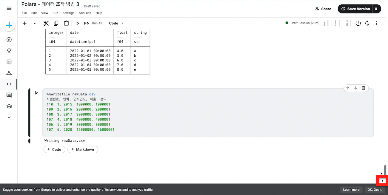
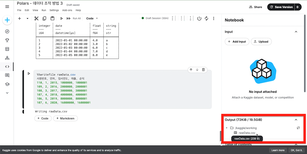
5.5 데이터 읽기
CSV 파일 데이터를 읽어와보도록 하겠습니다.
print(pl.read_csv('rawData.csv'))print(pl.read_csv('rawData.csv'))shape: (6, 5)
┌──────────┬──────┬──────────┬──────────┬─────────┐
│ 사원번호 ┆ 연차 ┆ 입사연도 ┆ 매출 ┆ 순익 │
│ --- ┆ --- ┆ --- ┆ --- ┆ --- │
│ i64 ┆ i64 ┆ i64 ┆ i64 ┆ i64 │
╞══════════╪══════╪══════════╪══════════╪═════════╡
│ 110 ┆ 1 ┆ 2015 ┆ 1000000 ┆ 100001 │
│ 109 ┆ 2 ┆ 2016 ┆ 2000000 ┆ 200001 │
│ 108 ┆ 3 ┆ 2017 ┆ 3000000 ┆ 300001 │
│ 107 ┆ 4 ┆ 2018 ┆ 4000000 ┆ 400001 │
│ 106 ┆ 5 ┆ 2019 ┆ 8000000 ┆ 800001 │
│ 107 ┆ 6 ┆ 2020 ┆ 16000000 ┆ 1600001 │
└──────────┴──────┴──────────┴──────────┴─────────┘shape: (6, 5)
┌──────────┬──────┬──────────┬──────────┬─────────┐
│ 사원번호 ┆ 연차 ┆ 입사연도 ┆ 매출 ┆ 순익 │
│ --- ┆ --- ┆ --- ┆ --- ┆ --- │
│ i64 ┆ i64 ┆ i64 ┆ i64 ┆ i64 │
╞══════════╪══════╪══════════╪══════════╪═════════╡
│ 110 ┆ 1 ┆ 2015 ┆ 1000000 ┆ 100001 │
│ 109 ┆ 2 ┆ 2016 ┆ 2000000 ┆ 200001 │
│ 108 ┆ 3 ┆ 2017 ┆ 3000000 ┆ 300001 │
│ 107 ┆ 4 ┆ 2018 ┆ 4000000 ┆ 400001 │
│ 106 ┆ 5 ┆ 2019 ┆ 8000000 ┆ 800001 │
│ 107 ┆ 6 ┆ 2020 ┆ 16000000 ┆ 1600001 │
└──────────┴──────┴──────────┴──────────┴─────────┘5.6 데이터 저장
데이터프레임을 CSV 파일로 저장해보도록 하겠습니다.
print(df.write_csv('df.csv'))print(df.write_csv('df.csv'))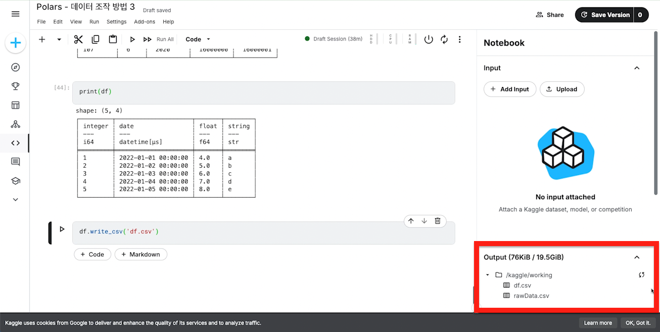
생성 또는 저장한 파일이 보이지 않는다면 🔁 새로고침 버튼을 클릭해주시길 바랍니다.
6. 데이터 삭제
데이터프레임에서 값을 삭제하는 방법은 여러 가지가 있습니다.
6.1 drop
drop 함수는 데이터프레임에서 지정한 열(컬럼)을 삭제할 때 사용하는 함수입니다. df.drop('a')을 이용해 ‘a’ 열을 삭제해보도록 하겠습니다.
# drop(’컬럼명’)
print(df.drop('a'))# drop(’컬럼명’)
print(df.drop('a'))shape: (5, 4)
┌─────┬─────────────────────┬───────┬───────┐
│ age ┆ date ┆ score ┆ grade │
│ --- ┆ --- ┆ --- ┆ --- │
│ i64 ┆ datetime[μs] ┆ f64 ┆ str │
╞═════╪═════════════════════╪═══════╪═══════╡
│ 10 ┆ 2022-01-01 00:00:00 ┆ 4.0 ┆ a │
│ 20 ┆ 2022-01-02 00:00:00 ┆ 5.0 ┆ b │
│ 30 ┆ 2022-01-03 00:00:00 ┆ 6.0 ┆ c │
│ 40 ┆ 2022-01-04 00:00:00 ┆ 7.0 ┆ b │
│ 50 ┆ 2022-01-05 00:00:00 ┆ 8.0 ┆ e │
└─────┴─────────────────────┴───────┴───────┘shape: (5, 4)
┌─────┬─────────────────────┬───────┬───────┐
│ age ┆ date ┆ score ┆ grade │
│ --- ┆ --- ┆ --- ┆ --- │
│ i64 ┆ datetime[μs] ┆ f64 ┆ str │
╞═════╪═════════════════════╪═══════╪═══════╡
│ 10 ┆ 2022-01-01 00:00:00 ┆ 4.0 ┆ a │
│ 20 ┆ 2022-01-02 00:00:00 ┆ 5.0 ┆ b │
│ 30 ┆ 2022-01-03 00:00:00 ┆ 6.0 ┆ c │
│ 40 ┆ 2022-01-04 00:00:00 ┆ 7.0 ┆ b │
│ 50 ┆ 2022-01-05 00:00:00 ┆ 8.0 ┆ e │
└─────┴─────────────────────┴───────┴───────┘한번 데이터프레임을 출력해보도록 하겠습니다. 출력 결과를 보시면 a열이 남아 있는 것을 보실 수 있습니다.
print(df)print(df)shape: (5, 5)
┌─────┬─────┬─────────────────────┬───────┬───────┐
│ a ┆ age ┆ date ┆ score ┆ grade │
│ --- ┆ --- ┆ --- ┆ --- ┆ --- │
│ i64 ┆ i64 ┆ datetime[μs] ┆ f64 ┆ str │
╞═════╪═════╪═════════════════════╪═══════╪═══════╡
│ 10 ┆ 10 ┆ 2022-01-01 00:00:00 ┆ 4.0 ┆ a │
│ 20 ┆ 20 ┆ 2022-01-02 00:00:00 ┆ 5.0 ┆ b │
│ 30 ┆ 30 ┆ 2022-01-03 00:00:00 ┆ 6.0 ┆ c │
│ 40 ┆ 40 ┆ 2022-01-04 00:00:00 ┆ 7.0 ┆ b │
│ 50 ┆ 50 ┆ 2022-01-05 00:00:00 ┆ 8.0 ┆ e │
└─────┴─────┴─────────────────────┴───────┴───────┘shape: (5, 5)
┌─────┬─────┬─────────────────────┬───────┬───────┐
│ a ┆ age ┆ date ┆ score ┆ grade │
│ --- ┆ --- ┆ --- ┆ --- ┆ --- │
│ i64 ┆ i64 ┆ datetime[μs] ┆ f64 ┆ str │
╞═════╪═════╪═════════════════════╪═══════╪═══════╡
│ 10 ┆ 10 ┆ 2022-01-01 00:00:00 ┆ 4.0 ┆ a │
│ 20 ┆ 20 ┆ 2022-01-02 00:00:00 ┆ 5.0 ┆ b │
│ 30 ┆ 30 ┆ 2022-01-03 00:00:00 ┆ 6.0 ┆ c │
│ 40 ┆ 40 ┆ 2022-01-04 00:00:00 ┆ 7.0 ┆ b │
│ 50 ┆ 50 ┆ 2022-01-05 00:00:00 ┆ 8.0 ┆ e │
└─────┴─────┴─────────────────────┴───────┴───────┘만약, 원본에 반영하고 싶다면 다시 df 변수에 저장해주어야 합니다. 실습 진행을 위해 실행시키지 않도록 하겠습니다.
# df = df.drop('a')
# print(df)# df = df.drop('a')
# print(df)여러 컬럼명을 연달아 작성하여 삭제하거나 리스트 형태로 작성하여 여러개의 컬럼을 삭제할 수 있습니다.
print(df.drop('a','score'))
# print(df.drop(['a','score']))print(df.drop('a','score'))
# print(df.drop(['a','score']))shape: (5, 3)
┌─────┬─────────────────────┬───────┐
│ age ┆ date ┆ grade │
│ --- ┆ --- ┆ --- │
│ i64 ┆ datetime[μs] ┆ str │
╞═════╪═════════════════════╪═══════╡
│ 10 ┆ 2022-01-01 00:00:00 ┆ a │
│ 20 ┆ 2022-01-02 00:00:00 ┆ b │
│ 30 ┆ 2022-01-03 00:00:00 ┆ c │
│ 40 ┆ 2022-01-04 00:00:00 ┆ b │
│ 50 ┆ 2022-01-05 00:00:00 ┆ e │
└─────┴─────────────────────┴───────┘shape: (5, 3)
┌─────┬─────────────────────┬───────┐
│ age ┆ date ┆ grade │
│ --- ┆ --- ┆ --- │
│ i64 ┆ datetime[μs] ┆ str │
╞═════╪═════════════════════╪═══════╡
│ 10 ┆ 2022-01-01 00:00:00 ┆ a │
│ 20 ┆ 2022-01-02 00:00:00 ┆ b │
│ 30 ┆ 2022-01-03 00:00:00 ┆ c │
│ 40 ┆ 2022-01-04 00:00:00 ┆ b │
│ 50 ┆ 2022-01-05 00:00:00 ┆ e │
└─────┴─────────────────────┴───────┘polars.selectors를 사용하여 여러개의 수치형 컬럼만 삭제할 수 있습니다. 출력 결과를 보시면 integer와 float가 삭제된 것을 볼 수 있습니다.
import polars.selectors as cs
print(df.drop(cs.numeric()))import polars.selectors as cs
print(df.drop(cs.numeric()))shape: (5, 2)
┌─────────────────────┬───────┐
│ date ┆ grade │
│ --- ┆ --- │
│ datetime[μs] ┆ str │
╞═════════════════════╪═══════╡
│ 2022-01-01 00:00:00 ┆ a │
│ 2022-01-02 00:00:00 ┆ b │
│ 2022-01-03 00:00:00 ┆ c │
│ 2022-01-04 00:00:00 ┆ b │
│ 2022-01-05 00:00:00 ┆ e │
└─────────────────────┴───────┘shape: (5, 2)
┌─────────────────────┬───────┐
│ date ┆ grade │
│ --- ┆ --- │
│ datetime[μs] ┆ str │
╞═════════════════════╪═══════╡
│ 2022-01-01 00:00:00 ┆ a │
│ 2022-01-02 00:00:00 ┆ b │
│ 2022-01-03 00:00:00 ┆ c │
│ 2022-01-04 00:00:00 ┆ b │
│ 2022-01-05 00:00:00 ┆ e │
└─────────────────────┴───────┘6.2 drop_in_place
단일 열을 삭제한 후 원본에 반영한 뒤, 삭제된 열을 반환합니다.
print(df.drop_in_place('a'))print(df.drop_in_place('a'))shape: (5,)
Series: 'a' [i64]
[
10
20
30
40
50
]shape: (5,)
Series: 'a' [i64]
[
10
20
30
40
50
]print(df)print(df)shape: (5, 4)
┌─────┬─────────────────────┬───────┬───────┐
│ age ┆ date ┆ score ┆ grade │
│ --- ┆ --- ┆ --- ┆ --- │
│ i64 ┆ datetime[μs] ┆ f64 ┆ str │
╞═════╪═════════════════════╪═══════╪═══════╡
│ 10 ┆ 2022-01-01 00:00:00 ┆ 4.0 ┆ a │
│ 20 ┆ 2022-01-02 00:00:00 ┆ 5.0 ┆ b │
│ 30 ┆ 2022-01-03 00:00:00 ┆ 6.0 ┆ c │
│ 40 ┆ 2022-01-04 00:00:00 ┆ 7.0 ┆ b │
│ 50 ┆ 2022-01-05 00:00:00 ┆ 8.0 ┆ e │
└─────┴─────────────────────┴───────┴───────┘
shape: (5, 4)
┌─────┬─────────────────────┬───────┬───────┐
│ age ┆ date ┆ score ┆ grade │
│ --- ┆ --- ┆ --- ┆ --- │
│ i64 ┆ datetime[μs] ┆ f64 ┆ str │
╞═════╪═════════════════════╪═══════╪═══════╡
│ 10 ┆ 2022-01-01 00:00:00 ┆ 4.0 ┆ a │
│ 20 ┆ 2022-01-02 00:00:00 ┆ 5.0 ┆ b │
│ 30 ┆ 2022-01-03 00:00:00 ┆ 6.0 ┆ c │
│ 40 ┆ 2022-01-04 00:00:00 ┆ 7.0 ┆ b │
│ 50 ┆ 2022-01-05 00:00:00 ┆ 8.0 ┆ e │
└─────┴─────────────────────┴───────┴───────┘
6.3 clear
데이터프레임 구조는 유지하면서 데이터만 지울 때 사용합니다.
print(df2)print(df2)shape: (2, 2)
┌──────┬──────┐
│ col1 ┆ col2 │
│ --- ┆ --- │
│ f32 ┆ i64 │
╞══════╪══════╡
│ 1.0 ┆ 3 │
│ 2.0 ┆ 4 │
└──────┴──────┘shape: (2, 2)
┌──────┬──────┐
│ col1 ┆ col2 │
│ --- ┆ --- │
│ f32 ┆ i64 │
╞══════╪══════╡
│ 1.0 ┆ 3 │
│ 2.0 ┆ 4 │
└──────┴──────┘먼저, 모든 데이터를 지우고 빈 데이터 프레임을 반환해보도록 하겠습니다. 이때, 컬럼명과 데이터 타입은 유지되며, 행의 수는 0이 됩니다.
print(df2.clear())print(df2.clear())shape: (0, 2)
┌──────┬──────┐
│ col1 ┆ col2 │
│ --- ┆ --- │
│ f32 ┆ i64 │
╞══════╪══════╡
└──────┴──────┘shape: (0, 2)
┌──────┬──────┐
│ col1 ┆ col2 │
│ --- ┆ --- │
│ f32 ┆ i64 │
╞══════╪══════╡
└──────┴──────┘지정된 n 크기만큼 null 값으로 채워진 행을 가진 데이터프레임을 생성해보도록 하겠습니다. 이때, n은 원본 데이터프레임 행의 수와 관계없이 원하는 크기로 지정할 수 있습니다.
print(df2.clear(n=2))print(df2.clear(n=2))shape: (2, 2)
┌──────┬──────┐
│ col1 ┆ col2 │
│ --- ┆ --- │
│ f32 ┆ i64 │
╞══════╪══════╡
│ null ┆ null │
│ null ┆ null │
└──────┴──────┘shape: (2, 2)
┌──────┬──────┐
│ col1 ┆ col2 │
│ --- ┆ --- │
│ f32 ┆ i64 │
╞══════╪══════╡
│ null ┆ null │
│ null ┆ null │
└──────┴──────┘7. 결측치 처리
7.1 결측값 추가
데이터프레임에 null 값을 추가하는 방법에 대해 알아보도록 하겠습니다.
df_null = pl.DataFrame({
'이름': ['A', 'B', None],
'나이': [25, 35, None],
'성별': ['남', '여', '남'],
'학점': [4.5, 4.0, None],
'주소': [None, 'jeju', None],
})
print(df_null)df_null = pl.DataFrame({
'이름': ['A', 'B', None],
'나이': [25, 35, None],
'성별': ['남', '여', '남'],
'학점': [4.5, 4.0, None],
'주소': [None, 'jeju', None],
})
print(df_null)shape: (3, 5)
┌──────┬──────┬──────┬──────┬──────┐
│ 이름 ┆ 나이 ┆ 성별 ┆ 학점 ┆ 주소 │
│ --- ┆ --- ┆ --- ┆ --- ┆ --- │
│ str ┆ i64 ┆ str ┆ f64 ┆ str │
╞══════╪══════╪══════╪══════╪══════╡
│ A ┆ 25 ┆ 남 ┆ 4.5 ┆ null │
│ B ┆ 35 ┆ 여 ┆ 4.0 ┆ jeju │
│ null ┆ null ┆ 남 ┆ null ┆ null │
└──────┴──────┴──────┴──────┴──────┘shape: (3, 5)
┌──────┬──────┬──────┬──────┬──────┐
│ 이름 ┆ 나이 ┆ 성별 ┆ 학점 ┆ 주소 │
│ --- ┆ --- ┆ --- ┆ --- ┆ --- │
│ str ┆ i64 ┆ str ┆ f64 ┆ str │
╞══════╪══════╪══════╪══════╪══════╡
│ A ┆ 25 ┆ 남 ┆ 4.5 ┆ null │
│ B ┆ 35 ┆ 여 ┆ 4.0 ┆ jeju │
│ null ┆ null ┆ 남 ┆ null ┆ null │
└──────┴──────┴──────┴──────┴──────┘데이터 값 추가했던 것과 같이 3번째 행, 성별 열에 None 값을 넣어주도록 하겠습니다.
df_null[2,'성별'] = None
print(df_null)df_null[2,'성별'] = None
print(df_null)shape: (3, 5)
┌──────┬──────┬──────┬──────┬──────┐
│ 이름 ┆ 나이 ┆ 성별 ┆ 학점 ┆ 주소 │
│ --- ┆ --- ┆ --- ┆ --- ┆ --- │
│ str ┆ i64 ┆ str ┆ f64 ┆ str │
╞══════╪══════╪══════╪══════╪══════╡
│ A ┆ 25 ┆ 남 ┆ 4.5 ┆ null │
│ B ┆ 35 ┆ 여 ┆ 4.0 ┆ jeju │
│ null ┆ null ┆ null ┆ null ┆ null │
└──────┴──────┴──────┴──────┴──────┘shape: (3, 5)
┌──────┬──────┬──────┬──────┬──────┐
│ 이름 ┆ 나이 ┆ 성별 ┆ 학점 ┆ 주소 │
│ --- ┆ --- ┆ --- ┆ --- ┆ --- │
│ str ┆ i64 ┆ str ┆ f64 ┆ str │
╞══════╪══════╪══════╪══════╪══════╡
│ A ┆ 25 ┆ 남 ┆ 4.5 ┆ null │
│ B ┆ 35 ┆ 여 ┆ 4.0 ┆ jeju │
│ null ┆ null ┆ null ┆ null ┆ null │
└──────┴──────┴──────┴──────┴──────┘이번에는 NaN 값을 추가하는 방법에 대해 알아보도록 하겠습니다.
df_nan = pl.DataFrame({
'이름': ['A', 'B', 'C'],
'나이': [25, 35, 40],
'성별': ['남', '여', '남'],
'학점': [4.5, 4.0, np.nan],
'주소': ['seoul', 'jeju', 'busan'],
})
print(df_nan)df_nan = pl.DataFrame({
'이름': ['A', 'B', 'C'],
'나이': [25, 35, 40],
'성별': ['남', '여', '남'],
'학점': [4.5, 4.0, np.nan],
'주소': ['seoul', 'jeju', 'busan'],
})
print(df_nan)- np.nan: NaN 값
shape: (3, 5)
┌──────┬──────┬──────┬──────┬───────┐
│ 이름 ┆ 나이 ┆ 성별 ┆ 학점 ┆ 주소 │
│ --- ┆ --- ┆ --- ┆ --- ┆ --- │
│ str ┆ i64 ┆ str ┆ f64 ┆ str │
╞══════╪══════╪══════╪══════╪═══════╡
│ A ┆ 25 ┆ 남 ┆ 4.5 ┆ seoul │
│ B ┆ 35 ┆ 여 ┆ 4.0 ┆ jeju │
│ C ┆ 40 ┆ 남 ┆ NaN ┆ busan │
└──────┴──────┴──────┴──────┴───────┘shape: (3, 5)
┌──────┬──────┬──────┬──────┬───────┐
│ 이름 ┆ 나이 ┆ 성별 ┆ 학점 ┆ 주소 │
│ --- ┆ --- ┆ --- ┆ --- ┆ --- │
│ str ┆ i64 ┆ str ┆ f64 ┆ str │
╞══════╪══════╪══════╪══════╪═══════╡
│ A ┆ 25 ┆ 남 ┆ 4.5 ┆ seoul │
│ B ┆ 35 ┆ 여 ┆ 4.0 ┆ jeju │
│ C ┆ 40 ┆ 남 ┆ NaN ┆ busan │
└──────┴──────┴──────┴──────┴───────┘아래와 같이 값을 NaN으로 변경할 경우 NaN값이 아닌, null 값이 들어가게 됩니다. 이는 NaN이 실수형이기 때문에 타입이 맞지 않아 null 값으로 들어가게 됩니다.
df_nan[1,1] = np.nan
print(df_nan)df_nan[1,1] = np.nan
print(df_nan)shape: (3, 5)
┌──────┬──────┬──────┬──────┬───────┐
│ 이름 ┆ 나이 ┆ 성별 ┆ 학점 ┆ 주소 │
│ --- ┆ --- ┆ --- ┆ --- ┆ --- │
│ str ┆ i64 ┆ str ┆ f64 ┆ str │
╞══════╪══════╪══════╪══════╪═══════╡
│ A ┆ 25 ┆ 남 ┆ 4.5 ┆ seoul │
│ B ┆ null ┆ 여 ┆ 4.0 ┆ jeju │
│ C ┆ 40 ┆ 남 ┆ NaN ┆ busan │
└──────┴──────┴──────┴──────┴───────┘shape: (3, 5)
┌──────┬──────┬──────┬──────┬───────┐
│ 이름 ┆ 나이 ┆ 성별 ┆ 학점 ┆ 주소 │
│ --- ┆ --- ┆ --- ┆ --- ┆ --- │
│ str ┆ i64 ┆ str ┆ f64 ┆ str │
╞══════╪══════╪══════╪══════╪═══════╡
│ A ┆ 25 ┆ 남 ┆ 4.5 ┆ seoul │
│ B ┆ null ┆ 여 ┆ 4.0 ┆ jeju │
│ C ┆ 40 ┆ 남 ┆ NaN ┆ busan │
└──────┴──────┴──────┴──────┴───────┘NaN 값을 추가할 때는 먼저 실수형으로 자료형을 변경한 뒤, NaN값으로 변경해주셔야 합니다.
df_nan = df_nan.cast({'나이':pl.Float32})
df_nan[1,1] = np.nan
print(df_nan)df_nan = df_nan.cast({'나이':pl.Float32})
df_nan[1,1] = np.nan
print(df_nan)shape: (3, 5)
┌──────┬──────┬──────┬──────┬───────┐
│ 이름 ┆ 나이 ┆ 성별 ┆ 학점 ┆ 주소 │
│ --- ┆ --- ┆ --- ┆ --- ┆ --- │
│ str ┆ f32 ┆ str ┆ f64 ┆ str │
╞══════╪══════╪══════╪══════╪═══════╡
│ A ┆ 25.0 ┆ 남 ┆ 4.5 ┆ seoul │
│ B ┆ NaN ┆ 여 ┆ 4.0 ┆ jeju │
│ C ┆ 40.0 ┆ 남 ┆ NaN ┆ busan │
└──────┴──────┴──────┴──────┴───────┘shape: (3, 5)
┌──────┬──────┬──────┬──────┬───────┐
│ 이름 ┆ 나이 ┆ 성별 ┆ 학점 ┆ 주소 │
│ --- ┆ --- ┆ --- ┆ --- ┆ --- │
│ str ┆ f32 ┆ str ┆ f64 ┆ str │
╞══════╪══════╪══════╪══════╪═══════╡
│ A ┆ 25.0 ┆ 남 ┆ 4.5 ┆ seoul │
│ B ┆ NaN ┆ 여 ┆ 4.0 ┆ jeju │
│ C ┆ 40.0 ┆ 남 ┆ NaN ┆ busan │
└──────┴──────┴──────┴──────┴───────┘7.2 결측치 확인
null_count는 데이터에 열별로 null 값의 개수가 몇개 있는지 확인할 수 있습니다.
print(df_null.null_count()) # 결측값 개수 확인print(df_null.null_count()) # 결측값 개수 확인shape: (1, 5)
┌──────┬──────┬──────┬──────┬──────┐
│ 이름 ┆ 나이 ┆ 성별 ┆ 학점 ┆ 주소 │
│ --- ┆ --- ┆ --- ┆ --- ┆ --- │
│ u32 ┆ u32 ┆ u32 ┆ u32 ┆ u32 │
╞══════╪══════╪══════╪══════╪══════╡
│ 1 ┆ 1 ┆ 1 ┆ 1 ┆ 2 │
└──────┴──────┴──────┴──────┴──────┘shape: (1, 5)
┌──────┬──────┬──────┬──────┬──────┐
│ 이름 ┆ 나이 ┆ 성별 ┆ 학점 ┆ 주소 │
│ --- ┆ --- ┆ --- ┆ --- ┆ --- │
│ u32 ┆ u32 ┆ u32 ┆ u32 ┆ u32 │
╞══════╪══════╪══════╪══════╪══════╡
│ 1 ┆ 1 ┆ 1 ┆ 1 ┆ 2 │
└──────┴──────┴──────┴──────┴──────┘7.3 결측치 처리
7.3.1 결측치 삭제(drop_nulls)
drop_nulls 함수는 데이터프레임에서 결측값(null)을 포함한 행을 삭제할 때 사용하는 함수입니다. drop_nulls 데이터프레임에서 첫번째, 세번째 주소 열에 null값이 포함되어 있으므로 두번째 행만 출력되는 것을 보실 수 있습니다.
print(df_null.drop_nulls())print(df_null.drop_nulls())shape: (1, 5)
┌──────┬──────┬──────┬──────┬──────┐
│ 이름 ┆ 나이 ┆ 성별 ┆ 학점 ┆ 주소 │
│ --- ┆ --- ┆ --- ┆ --- ┆ --- │
│ str ┆ i64 ┆ str ┆ f64 ┆ str │
╞══════╪══════╪══════╪══════╪══════╡
│ B ┆ 35 ┆ 여 ┆ 4.0 ┆ jeju │
└──────┴──────┴──────┴──────┴──────┘shape: (1, 5)
┌──────┬──────┬──────┬──────┬──────┐
│ 이름 ┆ 나이 ┆ 성별 ┆ 학점 ┆ 주소 │
│ --- ┆ --- ┆ --- ┆ --- ┆ --- │
│ str ┆ i64 ┆ str ┆ f64 ┆ str │
╞══════╪══════╪══════╪══════╪══════╡
│ B ┆ 35 ┆ 여 ┆ 4.0 ┆ jeju │
└──────┴──────┴──────┴──────┴──────┘subset 매개변수를 사용하여 polars 셀렉터로 데이터 타입이 문자열인 열이고 null이 있는 경우 행을 삭제해보도록 하겠습니다. 없음(기본값)으로 설정하면 모든 열에 있는 결측값을 확인하고 해당 행을 삭제합니다.
출력 결과를 보시면 문자열이 이름, 성별, 주소 열이 있는데 주소 열에 첫번째, 세번째 행에 null 값이 있으므로 삭제되고 출력된 것을 보실 수 있습니다.
print(df_null.drop_nulls(subset=cs.string()))print(df_null.drop_nulls(subset=cs.string()))shape: (1, 5)
┌──────┬──────┬──────┬──────┬──────┐
│ 이름 ┆ 나이 ┆ 성별 ┆ 학점 ┆ 주소 │
│ --- ┆ --- ┆ --- ┆ --- ┆ --- │
│ str ┆ i64 ┆ str ┆ f64 ┆ str │
╞══════╪══════╪══════╪══════╪══════╡
│ B ┆ 35 ┆ 여 ┆ 4.0 ┆ jeju │
└──────┴──────┴──────┴──────┴──────┘shape: (1, 5)
┌──────┬──────┬──────┬──────┬──────┐
│ 이름 ┆ 나이 ┆ 성별 ┆ 학점 ┆ 주소 │
│ --- ┆ --- ┆ --- ┆ --- ┆ --- │
│ str ┆ i64 ┆ str ┆ f64 ┆ str │
╞══════╪══════╪══════╪══════╪══════╡
│ B ┆ 35 ┆ 여 ┆ 4.0 ┆ jeju │
└──────┴──────┴──────┴──────┴──────┘모든 행이 null인 경우, 해당 행을 삭제해보도록 하겠습니다. 출력 결과를 보시면 모든 열이 null 값인 세번째 행을 제외하고 출력한 것을 보실 수 있습니다.
print(df_null.filter(~pl.all_horizontal(pl.all().is_null())))print(df_null.filter(~pl.all_horizontal(pl.all().is_null())))pl.all().is_null(): 모든 컬럼에 대한 각 값이 null 값이 있는지 조회합니다. null 값이 있으면 True, 아니면 False를 반환합니다.pl.all_horizontal(): 모든 행의 값이 채워져 있는지 확인합니다. 모든 행의 값이 null이면 True, 행의 값 중 하나라도 값이 있으면 False를 반환합니다.
shape: (2, 5)
┌──────┬──────┬──────┬──────┬──────┐
│ 이름 ┆ 나이 ┆ 성별 ┆ 학점 ┆ 주소 │
│ --- ┆ --- ┆ --- ┆ --- ┆ --- │
│ str ┆ i64 ┆ str ┆ f64 ┆ str │
╞══════╪══════╪══════╪══════╪══════╡
│ A ┆ 25 ┆ 남 ┆ 4.5 ┆ null │
│ B ┆ 35 ┆ 여 ┆ 4.0 ┆ jeju │
└──────┴──────┴──────┴──────┴──────┘shape: (2, 5)
┌──────┬──────┬──────┬──────┬──────┐
│ 이름 ┆ 나이 ┆ 성별 ┆ 학점 ┆ 주소 │
│ --- ┆ --- ┆ --- ┆ --- ┆ --- │
│ str ┆ i64 ┆ str ┆ f64 ┆ str │
╞══════╪══════╪══════╪══════╪══════╡
│ A ┆ 25 ┆ 남 ┆ 4.5 ┆ null │
│ B ┆ 35 ┆ 여 ┆ 4.0 ┆ jeju │
└──────┴──────┴──────┴──────┴──────┘모든 열이 null인 경우, 해당 열을 삭제해보도록 하겠습니다. 모든 열이 null인 경우를 만들어 주기 위해 두번째 행의 주소 열에 null 값을 채워보도록 하겠습니다.
df_null[1,'주소'] = None
print(df_null)df_null[1,'주소'] = None
print(df_null)shape: (3, 5)
┌──────┬──────┬──────┬──────┬──────┐
│ 이름 ┆ 나이 ┆ 성별 ┆ 학점 ┆ 주소 │
│ --- ┆ --- ┆ --- ┆ --- ┆ --- │
│ str ┆ i64 ┆ str ┆ f64 ┆ str │
╞══════╪══════╪══════╪══════╪══════╡
│ A ┆ 25 ┆ 남 ┆ 4.5 ┆ null │
│ B ┆ 35 ┆ 여 ┆ 4.0 ┆ null │
│ null ┆ null ┆ null ┆ null ┆ null │
└──────┴──────┴──────┴──────┴──────┘shape: (3, 5)
┌──────┬──────┬──────┬──────┬──────┐
│ 이름 ┆ 나이 ┆ 성별 ┆ 학점 ┆ 주소 │
│ --- ┆ --- ┆ --- ┆ --- ┆ --- │
│ str ┆ i64 ┆ str ┆ f64 ┆ str │
╞══════╪══════╪══════╪══════╪══════╡
│ A ┆ 25 ┆ 남 ┆ 4.5 ┆ null │
│ B ┆ 35 ┆ 여 ┆ 4.0 ┆ null │
│ null ┆ null ┆ null ┆ null ┆ null │
└──────┴──────┴──────┴──────┴──────┘데이터프레임을 순회하면서 컬럼명의 결측값의 개수가 데이터프레임의 길이와 동일한 경우를 제외한 컬럼명의 값들을 데이터프레임으로 반환합니다.
print(df_null[[s.name for s in df_null if not (s.null_count() == df_null.height)]])print(df_null[[s.name for s in df_null if not (s.null_count() == df_null.height)]])shape: (3, 4)
┌──────┬──────┬──────┬──────┐
│ 이름 ┆ 나이 ┆ 성별 ┆ 학점 │
│ --- ┆ --- ┆ --- ┆ --- │
│ str ┆ i64 ┆ str ┆ f64 │
╞══════╪══════╪══════╪══════╡
│ A ┆ 25 ┆ 남 ┆ 4.5 │
│ B ┆ 35 ┆ 여 ┆ 4.0 │
│ null ┆ null ┆ null ┆ null │
└──────┴──────┴──────┴──────┘shape: (3, 4)
┌──────┬──────┬──────┬──────┐
│ 이름 ┆ 나이 ┆ 성별 ┆ 학점 │
│ --- ┆ --- ┆ --- ┆ --- │
│ str ┆ i64 ┆ str ┆ f64 │
╞══════╪══════╪══════╪══════╡
│ A ┆ 25 ┆ 남 ┆ 4.5 │
│ B ┆ 35 ┆ 여 ┆ 4.0 │
│ null ┆ null ┆ null ┆ null │
└──────┴──────┴──────┴──────┘7.3.2 결측치 채우기(fill_null, fill_nan)
fill_null을 사용하여 지정된 값이나 어떤 값을 채울지 전략을 세워 null 값을 채울 수 있습니다.
- value : null 값 대신 채울 값
- strategy : null 값을 채우는 데 사용되는 전략
- None(기본값), forward, backward, min, max, mean, 0, 1
- limit : strategy에서 'forward' 또는 'backward'를 사용할 때 연속으로 채울 null 값의 개수
- matches_supertype : 채울 값의 타입이 다를 경우, 채울 값의 타입과 일치하도록 열의 타입을 채울 값의 타입으로 변경합니다. 기본값은 True이며, False로 설정할 경우 타입이 맞는 열에만 값이 채워지며, 타입이 맞지 않은 열은 null을 출력하게 됩니다.
결측값을 99라는 값으로 채워보도록 하겠습니다. 출력 결과를 보시면, 수치형 변수의 결측치에 99로 채워진 것을 보실 수 있습니다.
print(df_null.fill_null(99))print(df_null.fill_null(99))shape: (3, 5)
┌──────┬──────┬──────┬──────┬──────┐
│ 이름 ┆ 나이 ┆ 성별 ┆ 학점 ┆ 주소 │
│ --- ┆ --- ┆ --- ┆ --- ┆ --- │
│ str ┆ i64 ┆ str ┆ f64 ┆ str │
╞══════╪══════╪══════╪══════╪══════╡
│ A ┆ 25 ┆ 남 ┆ 4.5 ┆ null │
│ B ┆ 35 ┆ 여 ┆ 4.0 ┆ null │
│ null ┆ 99 ┆ null ┆ 99.0 ┆ null │
└──────┴──────┴──────┴──────┴──────┘shape: (3, 5)
┌──────┬──────┬──────┬──────┬──────┐
│ 이름 ┆ 나이 ┆ 성별 ┆ 학점 ┆ 주소 │
│ --- ┆ --- ┆ --- ┆ --- ┆ --- │
│ str ┆ i64 ┆ str ┆ f64 ┆ str │
╞══════╪══════╪══════╪══════╪══════╡
│ A ┆ 25 ┆ 남 ┆ 4.5 ┆ null │
│ B ┆ 35 ┆ 여 ┆ 4.0 ┆ null │
│ null ┆ 99 ┆ null ┆ 99.0 ┆ null │
└──────┴──────┴──────┴──────┴──────┘만약, 문자열의 결측치를 채우고 싶으시다면 value에 문자열 형태의 값을 넣어주시면 됩니다. 한번 ‘X’로 채워보도록 하겠습니다.
print(df_null.fill_null('X'))print(df_null.fill_null('X'))shape: (3, 5)
┌──────┬──────┬──────┬──────┬──────┐
│ 이름 ┆ 나이 ┆ 성별 ┆ 학점 ┆ 주소 │
│ --- ┆ --- ┆ --- ┆ --- ┆ --- │
│ str ┆ i64 ┆ str ┆ f64 ┆ str │
╞══════╪══════╪══════╪══════╪══════╡
│ A ┆ 25 ┆ 남 ┆ 4.5 ┆ X │
│ B ┆ 35 ┆ 여 ┆ 4.0 ┆ X │
│ X ┆ null ┆ X ┆ null ┆ X │
└──────┴──────┴──────┴──────┴──────┘shape: (3, 5)
┌──────┬──────┬──────┬──────┬──────┐
│ 이름 ┆ 나이 ┆ 성별 ┆ 학점 ┆ 주소 │
│ --- ┆ --- ┆ --- ┆ --- ┆ --- │
│ str ┆ i64 ┆ str ┆ f64 ┆ str │
╞══════╪══════╪══════╪══════╪══════╡
│ A ┆ 25 ┆ 남 ┆ 4.5 ┆ X │
│ B ┆ 35 ┆ 여 ┆ 4.0 ┆ X │
│ X ┆ null ┆ X ┆ null ┆ X │
└──────┴──────┴──────┴──────┴──────┘이번에는 strategy 매개변수를 사용하여 각 열의 최댓값으로 채워주도록 하겠습니다. 출력 결과를 보시면 null를 제외한 값 중 최대값으로 결측값을 채워진 것을 볼 수 있습니다.
print(df_null['나이','학점'].fill_null(strategy="max"))print(df_null['나이','학점'].fill_null(strategy="max"))shape: (3, 2)
┌──────┬──────┐
│ 나이 ┆ 학점 │
│ --- ┆ --- │
│ i64 ┆ f64 │
╞══════╪══════╡
│ 25 ┆ 4.5 │
│ 35 ┆ 4.0 │
│ 35 ┆ 4.5 │
└──────┴──────┘shape: (3, 2)
┌──────┬──────┐
│ 나이 ┆ 학점 │
│ --- ┆ --- │
│ i64 ┆ f64 │
╞══════╪══════╡
│ 25 ┆ 4.5 │
│ 35 ┆ 4.0 │
│ 35 ┆ 4.5 │
└──────┴──────┘이번에는 결측값을 0으로 채워보도록 하겠습니다.
print(df_null['나이','학점'].fill_null(strategy="zero"))print(df_null['나이','학점'].fill_null(strategy="zero"))shape: (3, 2)
┌──────┬──────┐
│ 나이 ┆ 학점 │
│ --- ┆ --- │
│ i64 ┆ f64 │
╞══════╪══════╡
│ 25 ┆ 4.5 │
│ 35 ┆ 4.0 │
│ 0 ┆ 0.0 │
└──────┴──────┘shape: (3, 2)
┌──────┬──────┐
│ 나이 ┆ 학점 │
│ --- ┆ --- │
│ i64 ┆ f64 │
╞══════╪══════╡
│ 25 ┆ 4.5 │
│ 35 ┆ 4.0 │
│ 0 ┆ 0.0 │
└──────┴──────┘이번에는 null 값의 앞에 있는 값으로 채워보도록 하겠습니다. 출력 결과를 보시면 나이는 35로 학점은 4.0으로 채워진 것을 볼 수 있습니다.
print(df_null['나이','학점'].fill_null(strategy="forward"))print(df_null['나이','학점'].fill_null(strategy="forward"))shape: (3, 2)
┌──────┬──────┐
│ 나이 ┆ 학점 │
│ --- ┆ --- │
│ i64 ┆ f64 │
╞══════╪══════╡
│ 25 ┆ 4.5 │
│ 35 ┆ 4.0 │
│ 35 ┆ 4.0 │
└──────┴──────┘shape: (3, 2)
┌──────┬──────┐
│ 나이 ┆ 학점 │
│ --- ┆ --- │
│ i64 ┆ f64 │
╞══════╪══════╡
│ 25 ┆ 4.5 │
│ 35 ┆ 4.0 │
│ 35 ┆ 4.0 │
└──────┴──────┘strategy에서 forward, backward로 채울 때 연속으로 채울 null 값의 개수를 설정할 수 있습니다. limit를 1로 설정하여 null 값 하나를 앞에 있는 값으로 채운것을 볼 수 있습니다.
print(df_null['나이','학점'].fill_null(strategy="forward", limit=1))print(df_null['나이','학점'].fill_null(strategy="forward", limit=1))shape: (3, 2)
┌──────┬──────┐
│ 나이 ┆ 학점 │
│ --- ┆ --- │
│ i64 ┆ f64 │
╞══════╪══════╡
│ 25 ┆ 4.5 │
│ 35 ┆ 4.0 │
│ 35 ┆ 4.0 │
└──────┴──────┘shape: (3, 2)
┌──────┬──────┐
│ 나이 ┆ 학점 │
│ --- ┆ --- │
│ i64 ┆ f64 │
╞══════╪══════╡
│ 25 ┆ 4.5 │
│ 35 ┆ 4.0 │
│ 35 ┆ 4.0 │
└──────┴──────┘이번에는 matches_supertype 매개변수를 사용하여 채울 값의 데이터 타입이 다른 경우 채울 값의 일치하도록 열의 타입을 변경해보도록 하겠습니다. 기본값은 True이며, False로 설정한 경우 타입이 맞는 열에만 값을 채울 수 있습니다.
나이, 학점에 9.9를 채워보도록 하겠습니다. 출력 결과를 보시면 나이 열이 실수형으로 바뀐 것을 볼 수 있습니다.
print(df_null['나이','학점'].fill_null(9.9, matches_supertype=True))print(df_null['나이','학점'].fill_null(9.9, matches_supertype=True))shape: (3, 2)
┌──────┬──────┐
│ 나이 ┆ 학점 │
│ --- ┆ --- │
│ f64 ┆ f64 │
╞══════╪══════╡
│ 25.0 ┆ 4.5 │
│ 35.0 ┆ 4.0 │
│ 9.9 ┆ 9.9 │
└──────┴──────┘shape: (3, 2)
┌──────┬──────┐
│ 나이 ┆ 학점 │
│ --- ┆ --- │
│ f64 ┆ f64 │
╞══════╪══════╡
│ 25.0 ┆ 4.5 │
│ 35.0 ┆ 4.0 │
│ 9.9 ┆ 9.9 │
└──────┴──────┘이번에는 matches_supertype를 False로 설정하여 채울 값의 타입과 맞는 열에만 값을 채워보도록 하겠습니다. 출력 결과를 보시면 나이 열의 타입은 정수형이기 때문에 null 값이 채워진 것을 볼 수 있습니다.
print(df_null['나이','학점'].fill_null(9.9, matches_supertype=False))print(df_null['나이','학점'].fill_null(9.9, matches_supertype=False))shape: (3, 2)
┌──────┬──────┐
│ 나이 ┆ 학점 │
│ --- ┆ --- │
│ i64 ┆ f64 │
╞══════╪══════╡
│ 25 ┆ 4.5 │
│ 35 ┆ 4.0 │
│ null ┆ 9.9 │
└──────┴──────┘shape: (3, 2)
┌──────┬──────┐
│ 나이 ┆ 학점 │
│ --- ┆ --- │
│ i64 ┆ f64 │
╞══════╪══════╡
│ 25 ┆ 4.5 │
│ 35 ┆ 4.0 │
│ null ┆ 9.9 │
└──────┴──────┘fill_nan을 사용하여 부동 소수점 NaN 값을 다른 값으로 채울 수 있습니다. 출력해보시면, NaN 값에 3.5가 채워진 것을 보실 수 있습니다.
print(df_nan.fill_nan(3.5))print(df_nan.fill_nan(3.5))shape: (3, 5)
┌──────┬──────┬──────┬──────┬───────┐
│ 이름 ┆ 나이 ┆ 성별 ┆ 학점 ┆ 주소 │
│ --- ┆ --- ┆ --- ┆ --- ┆ --- │
│ str ┆ f32 ┆ str ┆ f64 ┆ str │
╞══════╪══════╪══════╪══════╪═══════╡
│ A ┆ 25.0 ┆ 남 ┆ 4.5 ┆ seoul │
│ B ┆ 3.5 ┆ 여 ┆ 4.0 ┆ jeju │
│ C ┆ 40.0 ┆ 남 ┆ 3.5 ┆ busan │
└──────┴──────┴──────┴──────┴───────┘shape: (3, 5)
┌──────┬──────┬──────┬──────┬───────┐
│ 이름 ┆ 나이 ┆ 성별 ┆ 학점 ┆ 주소 │
│ --- ┆ --- ┆ --- ┆ --- ┆ --- │
│ str ┆ f32 ┆ str ┆ f64 ┆ str │
╞══════╪══════╪══════╪══════╪═══════╡
│ A ┆ 25.0 ┆ 남 ┆ 4.5 ┆ seoul │
│ B ┆ 3.5 ┆ 여 ┆ 4.0 ┆ jeju │
│ C ┆ 40.0 ┆ 남 ┆ 3.5 ┆ busan │
└──────┴──────┴──────┴──────┴───────┘부동소수점 NaN(숫자 아님)은 누락된 값이 아니라는 점에 유의하셔야 합니다. 누락된 값을 대체하려면 fill_null()을 사용하는 것을 권장합니다.
8. 데이터 필터
8.1 filter
filter 메서드는 하나 이상의 조건을 기준으로 데이터프레임의 행을 필터링합니다. 필터링 결과는 논리형(True, Fasle) 시리즈로 True로 반환된 행만 출력되며, False로 반환된 행은 null을 포함하여 삭제됩니다. 이때, 행의 순서는 기존 데이터프레임과 같은 순서대로 유지됩니다.
실습을 위해 데이터프레임을 생성하고 foo 열의 값이 1보다 큰 값을 가진 행을 조회해보도록 하겠습니다.
df = pl.DataFrame(
{
"foo": [1, 2, 3],
"bar": [6, 7, 8],
"ham": ["a", "b", "c"],
}
)
# df.filter(필터링 할 조건)
print(df.filter(pl.col("foo") > 1))df = pl.DataFrame(
{
"foo": [1, 2, 3],
"bar": [6, 7, 8],
"ham": ["a", "b", "c"],
}
)
# df.filter(필터링 할 조건)
print(df.filter(pl.col("foo") > 1))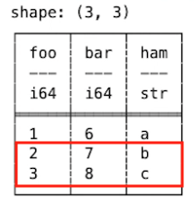
shape: (2, 3)
┌─────┬─────┬─────┐
│ foo ┆ bar ┆ ham │
│ --- ┆ --- ┆ --- │
│ i64 ┆ i64 ┆ str │
╞═════╪═════╪═════╡
│ 2 ┆ 7 ┆ b │
│ 3 ┆ 8 ┆ c │
└─────┴─────┴─────┘shape: (2, 3)
┌─────┬─────┬─────┐
│ foo ┆ bar ┆ ham │
│ --- ┆ --- ┆ --- │
│ i64 ┆ i64 ┆ str │
╞═════╪═════╪═════╡
│ 2 ┆ 7 ┆ b │
│ 3 ┆ 8 ┆ c │
└─────┴─────┴─────┘조건을 여러개 두고 싶은 경우, &(and, 그리고) 연산자, |(or, 또는) 연산자, ~(not, 아닌) 연산자와 결합하여 필터링 할 수 있습니다.
and 연산자를 사용하여 foo가 3 미만이고, ham이 a인 행을 출력해보도록 하겠습니다.
print(df.filter((pl.col("foo") < 3) & (pl.col("ham") == "a")))print(df.filter((pl.col("foo") < 3) & (pl.col("ham") == "a")))shape: (1, 3)
┌─────┬─────┬─────┐
│ foo ┆ bar ┆ ham │
│ --- ┆ --- ┆ --- │
│ i64 ┆ i64 ┆ str │
╞═════╪═════╪═════╡
│ 1 ┆ 6 ┆ a │
└─────┴─────┴─────┘shape: (1, 3)
┌─────┬─────┬─────┐
│ foo ┆ bar ┆ ham │
│ --- ┆ --- ┆ --- │
│ i64 ┆ i64 ┆ str │
╞═════╪═════╪═════╡
│ 1 ┆ 6 ┆ a │
└─────┴─────┴─────┘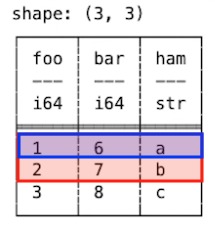
or 연산자를 사용하여 foo가 1이거나 ham이 c인 행을 출력해보도록 하겠습니다.
print(df.filter((pl.col("foo") == 1) | (pl.col("ham") == "c")))print(df.filter((pl.col("foo") == 1) | (pl.col("ham") == "c")))shape: (2, 3)
┌─────┬─────┬─────┐
│ foo ┆ bar ┆ ham │
│ --- ┆ --- ┆ --- │
│ i64 ┆ i64 ┆ str │
╞═════╪═════╪═════╡
│ 1 ┆ 6 ┆ a │
│ 3 ┆ 8 ┆ c │
└─────┴─────┴─────┘shape: (2, 3)
┌─────┬─────┬─────┐
│ foo ┆ bar ┆ ham │
│ --- ┆ --- ┆ --- │
│ i64 ┆ i64 ┆ str │
╞═════╪═════╪═════╡
│ 1 ┆ 6 ┆ a │
│ 3 ┆ 8 ┆ c │
└─────┴─────┴─────┘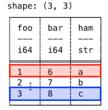
not 연산자를 사용하여 foo가 2 이하이고 ham에 b와 c의 값이 들어가지 않은 행을 출력해보도록 하겠습니다. 이때, 조건을 쉼표(,)로 연결하여 and 연산자와 같이 여러 조건을 모두 만족하는 행을 출력할 수 있습니다.
print(df.filter(
pl.col("foo") <= 2,
~pl.col("ham").is_in(["b", "c"]),
))print(df.filter(
pl.col("foo") <= 2,
~pl.col("ham").is_in(["b", "c"]),
))- is_in([’값1’,’값2’]) : 리스트 안에 있는 값이 들어간 경우만 출력합니다.
shape: (1, 3)
┌─────┬─────┬─────┐
│ foo ┆ bar ┆ ham │
│ --- ┆ --- ┆ --- │
│ i64 ┆ i64 ┆ str │
╞═════╪═════╪═════╡
│ 1 ┆ 6 ┆ a │
└─────┴─────┴─────┘shape: (1, 3)
┌─────┬─────┬─────┐
│ foo ┆ bar ┆ ham │
│ --- ┆ --- ┆ --- │
│ i64 ┆ i64 ┆ str │
╞═════╪═════╪═════╡
│ 1 ┆ 6 ┆ a │
└─────┴─────┴─────┘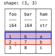
컬럼명에 값을 매핑하여(컬럼명 = 값) 필터링을 해보도록 하겠습니다. pl.col(name).eq(value)와 동일하게 작동합니다. foo가 2이고 ham이 b인 행을 출력해보도록 하겠습니다.
print(df.filter(foo=2, ham="b"))print(df.filter(foo=2, ham="b"))shape: (1, 3)
┌─────┬─────┬─────┐
│ foo ┆ bar ┆ ham │
│ --- ┆ --- ┆ --- │
│ i64 ┆ i64 ┆ str │
╞═════╪═════╪═════╡
│ 2 ┆ 7 ┆ b │
└─────┴─────┴─────┘shape: (1, 3)
┌─────┬─────┬─────┐
│ foo ┆ bar ┆ ham │
│ --- ┆ --- ┆ --- │
│ i64 ┆ i64 ┆ str │
╞═════╪═════╪═════╡
│ 2 ┆ 7 ┆ b │
└─────┴─────┴─────┘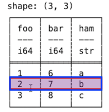
8.2 is_duplicated
is_duplicated 메서드는 데이터프레임에서 중복된 모든 행의 논리형(bool) 값을 가져옵니다. 실습에 들어가기에 앞서 데이터프레임을 생성해보도록 하겠습니다.
df = pl.DataFrame(
{
"a": [1, 2, 3, 1],
"b": ["x", "y", "z", "x"],
"c": ["b", "b", "b", "b"],
}
)
print(df)df = pl.DataFrame(
{
"a": [1, 2, 3, 1],
"b": ["x", "y", "z", "x"],
"c": ["b", "b", "b", "b"],
}
)
print(df)shape: (4, 3)
┌─────┬─────┬─────┐
│ a ┆ b ┆ c │
│ --- ┆ --- ┆ --- │
│ i64 ┆ str ┆ str │
╞═════╪═════╪═════╡
│ 1 ┆ x ┆ b │
│ 2 ┆ y ┆ b │
│ 3 ┆ z ┆ b │
│ 1 ┆ x ┆ b │
└─────┴─────┴─────┘shape: (4, 3)
┌─────┬─────┬─────┐
│ a ┆ b ┆ c │
│ --- ┆ --- ┆ --- │
│ i64 ┆ str ┆ str │
╞═════╪═════╪═════╡
│ 1 ┆ x ┆ b │
│ 2 ┆ y ┆ b │
│ 3 ┆ z ┆ b │
│ 1 ┆ x ┆ b │
└─────┴─────┴─────┘데이터프레임에서 중복된 행이 있는지 확인해보도록 하겠습니다. 출력 결과를 보시면 첫번째, 마지막 행의 값이 동일하기 때문에 중복된 행은 True, 중복되지 않은 행은 False로 출력된 것을 보실 수 있습니다.
print(df.is_duplicated())print(df.is_duplicated())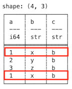
shape: (4,)
Series: '' [bool]
[
true
false
false
true
]shape: (4,)
Series: '' [bool]
[
true
false
false
true
]만약, 중복된 행의 데이터를 출력하고 싶으시다면 filter 메서드와 함께 사용하시면 됩니다.
print(df.filter(df.is_duplicated()))print(df.filter(df.is_duplicated()))shape: (2, 3)
┌─────┬─────┬─────┐
│ a ┆ b ┆ c │
│ --- ┆ --- ┆ --- │
│ i64 ┆ str ┆ str │
╞═════╪═════╪═════╡
│ 1 ┆ x ┆ b │
│ 1 ┆ x ┆ b │
└─────┴─────┴─────┘shape: (2, 3)
┌─────┬─────┬─────┐
│ a ┆ b ┆ c │
│ --- ┆ --- ┆ --- │
│ i64 ┆ str ┆ str │
╞═════╪═════╪═════╡
│ 1 ┆ x ┆ b │
│ 1 ┆ x ┆ b │
└─────┴─────┴─────┘8.3 is_unique
is_unique 메서드는 데이터프레임의 모든 고유한 행을 가지고 있는지 확인합니다. 출력 결과를 보시면 두번째, 세번째 행은 고유한 값을 가지므로 True로 출력된 것을 보실 수 있고, 중복된 행은 False로 출력됩니다.
print(df.is_unique())print(df.is_unique())shape: (4,)
Series: '' [bool]
[
false
true
true
false
]shape: (4,)
Series: '' [bool]
[
false
true
true
false
]고유값을 가진 행의 데이터를 출력해보도록 하겠습니다.
print(df.filter(df.is_unique()))print(df.filter(df.is_unique()))shape: (2, 3)
┌─────┬─────┬─────┐
│ a ┆ b ┆ c │
│ --- ┆ --- ┆ --- │
│ i64 ┆ str ┆ str │
╞═════╪═════╪═════╡
│ 2 ┆ y ┆ b │
│ 3 ┆ z ┆ b │
└─────┴─────┴─────┘shape: (2, 3)
┌─────┬─────┬─────┐
│ a ┆ b ┆ c │
│ --- ┆ --- ┆ --- │
│ i64 ┆ str ┆ str │
╞═════╪═════╪═════╡
│ 2 ┆ y ┆ b │
│ 3 ┆ z ┆ b │
└─────┴─────┴─────┘8.4 unique
unique 메서드는 데이터프레임에서 중복된 행을 삭제합니다. 만약, 데이터프레임 또는 하위 집합에 List 유형의 열이 있는 경우 이 메서드는 동작하지 않습니다. 출력 결과를 보면 중복된 행(1, a, b)은 하나만 출력된 것을 보실 수 있습니다. 즉, unique 메서드는 고유한 값만 출력합니다.
print(df.unique())print(df.unique())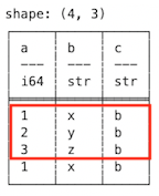
shape: (3, 3)
┌─────┬─────┬─────┐
│ a ┆ b ┆ c │
│ --- ┆ --- ┆ --- │
│ i64 ┆ str ┆ str │
╞═════╪═════╪═════╡
│ 2 ┆ y ┆ b │
│ 1 ┆ x ┆ b │
│ 3 ┆ z ┆ b │
└─────┴─────┴─────┘shape: (3, 3)
┌─────┬─────┬─────┐
│ a ┆ b ┆ c │
│ --- ┆ --- ┆ --- │
│ i64 ┆ str ┆ str │
╞═════╪═════╪═════╡
│ 2 ┆ y ┆ b │
│ 1 ┆ x ┆ b │
│ 3 ┆ z ┆ b │
└─────┴─────┴─────┘- subset : 중복 행을 식별할 때 고려할 컬럼명을 선택합니다. 없음(기본값)으로 설정하면 모든 열을 사용합니다.
- keep : 중복 행 중 어떤 행을 유지할지 설정합니다.
- 'any': 어떤 행이 유지되는지 보장하지 않고 더 많은 최적화가 가능합니다.
- 'none': 중복 행을 유지하지 않습니다.
- 'first': 중복 행 중 첫 번째 고유 행을 유지합니다.
- 'last': 중복 행 중 마지막 고유 행을 유지합니다.
- maintain_order : 원래 데이터프레임과 동일한 순서를 유지합니다. 이 경우 계산 비용이 더 많이 듭니다. True로 설정하면 스트리밍 엔진에서 실행할 가능성이 차단됩니다.
subset 매개변수를 설정하여 b와 c열에 있는 값을 결합한 후에 고유값을 가진 행을 출력해보도록 하겠습니다. 출력 결과를 보시면 중복된 행 중 가장 먼저 생성된 데이터가 출력된 것을 보실 수 있습니다.
print(df.unique(subset=["b", "c"]))print(df.unique(subset=["b", "c"]))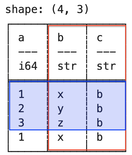
shape: (3, 3)
┌─────┬─────┬─────┐
│ a ┆ b ┆ c │
│ --- ┆ --- ┆ --- │
│ i64 ┆ str ┆ str │
╞═════╪═════╪═════╡
│ 1 ┆ x ┆ b │
│ 2 ┆ y ┆ b │
│ 3 ┆ z ┆ b │
└─────┴─────┴─────┘shape: (3, 3)
┌─────┬─────┬─────┐
│ a ┆ b ┆ c │
│ --- ┆ --- ┆ --- │
│ i64 ┆ str ┆ str │
╞═════╪═════╪═════╡
│ 1 ┆ x ┆ b │
│ 2 ┆ y ┆ b │
│ 3 ┆ z ┆ b │
└─────┴─────┴─────┘keep 매개변수를 last로 설정하여 중복 행 중 마지막 행을 유지해보도록 하겠습니다.
print(df.unique(keep="last"))print(df.unique(keep="last"))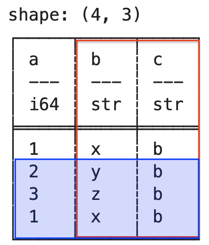
shape: (3, 3)
┌─────┬─────┬─────┐
│ a ┆ b ┆ c │
│ --- ┆ --- ┆ --- │
│ i64 ┆ str ┆ str │
╞═════╪═════╪═════╡
│ 1 ┆ x ┆ b │
│ 2 ┆ y ┆ b │
│ 3 ┆ z ┆ b │
└─────┴─────┴─────┘shape: (3, 3)
┌─────┬─────┬─────┐
│ a ┆ b ┆ c │
│ --- ┆ --- ┆ --- │
│ i64 ┆ str ┆ str │
╞═════╪═════╪═════╡
│ 1 ┆ x ┆ b │
│ 2 ┆ y ┆ b │
│ 3 ┆ z ┆ b │
└─────┴─────┴─────┘maintain_order 매개변수를 True로 설정하여 원래 데이터프레임과 동일한 순서를 유지하여 출력된 것을 보실 수 있습니다.
print(df.unique(subset=["b", "c"], maintain_order=True))print(df.unique(subset=["b", "c"], maintain_order=True))shape: (3, 3)
┌─────┬─────┬─────┐
│ a ┆ b ┆ c │
│ --- ┆ --- ┆ --- │
│ i64 ┆ str ┆ str │
╞═════╪═════╪═════╡
│ 1 ┆ x ┆ b │
│ 2 ┆ y ┆ b │
│ 3 ┆ z ┆ b │
└─────┴─────┴─────┘shape: (3, 3)
┌─────┬─────┬─────┐
│ a ┆ b ┆ c │
│ --- ┆ --- ┆ --- │
│ i64 ┆ str ┆ str │
╞═════╪═════╪═════╡
│ 1 ┆ x ┆ b │
│ 2 ┆ y ┆ b │
│ 3 ┆ z ┆ b │
└─────┴─────┴─────┘pandas의 drop_duplicates와 유사합니다.
특정 컬럼 중에서 고유값을 출력해보도록 하겠습니다. 출력 결과를 보시면 a 열에 1,2,3이라는 고유값이 있는 것을 확인할 수 있습니다.
print(df["a"].unique())print(df["a"].unique())shape: (3,)
Series: 'a' [i64]
[
1
2
3
]shape: (3,)
Series: 'a' [i64]
[
1
2
3
]8.5 n_unique
n_unique 메서드는 고유한 행의 수 또는 고유한 행 부분 집합의 수를 반환합니다. 먼저, 실습에 필요한 데이터프레임을 생성해주도록 하겠습니다.
df = pl.DataFrame(
{
"a": [1, 1, 2, 3, 4, 5],
"b": [0.5, 0.5, 1.0, 2.0, 3.0, 3.0],
"c": [True, True, True, False, True, True],
}
)
print(df)df = pl.DataFrame(
{
"a": [1, 1, 2, 3, 4, 5],
"b": [0.5, 0.5, 1.0, 2.0, 3.0, 3.0],
"c": [True, True, True, False, True, True],
}
)
print(df)shape: (6, 3)
┌─────┬─────┬───────┐
│ a ┆ b ┆ c │
│ --- ┆ --- ┆ --- │
│ i64 ┆ f64 ┆ bool │
╞═════╪═════╪═══════╡
│ 1 ┆ 0.5 ┆ true │
│ 1 ┆ 0.5 ┆ true │
│ 2 ┆ 1.0 ┆ true │
│ 3 ┆ 2.0 ┆ false │
│ 4 ┆ 3.0 ┆ true │
│ 5 ┆ 3.0 ┆ true │
└─────┴─────┴───────┘shape: (6, 3)
┌─────┬─────┬───────┐
│ a ┆ b ┆ c │
│ --- ┆ --- ┆ --- │
│ i64 ┆ f64 ┆ bool │
╞═════╪═════╪═══════╡
│ 1 ┆ 0.5 ┆ true │
│ 1 ┆ 0.5 ┆ true │
│ 2 ┆ 1.0 ┆ true │
│ 3 ┆ 2.0 ┆ false │
│ 4 ┆ 3.0 ┆ true │
│ 5 ┆ 3.0 ┆ true │
└─────┴─────┴───────┘n_unique를 사용하여 고유한 행의 수를 출력해보도록 하겠습니다. 5가 출력된 것을 보실 수 있는데 데이터프레임의 첫번째, 두번째 행이 중복되므로 총 5개의 고유한 행이 있는 것을 확인하실 수 있습니다.
print(df.n_unique())print(df.n_unique())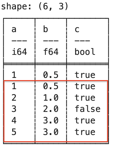
55특정 컬럼 값에 고유값 개수를 확인해보도록 하겠습니다. 출력 결과를 보시면 c 열에는 3개의 고유값이 있는 것을 확인하실 수 있습니다.
print(df['c'].n_unique())print(df['c'].n_unique())
22n_unique 메서드도 subset 매개변수를 사용하여 여러 열을 결합하여 고유값의 개수를 확인하실 수 있습니다. 출력 결과를 보시면 b와 c열을 결합한 결과 고유값이 4개가 있는 것을 보실 수 있습니다.
# 단순 열
print(df.n_unique(subset=["b", "c"]))# 단순 열
print(df.n_unique(subset=["b", "c"]))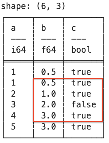
44이번에는 subset 매개변수에 표현식을 작성해보도록 하겠습니다. a열을 2로 나누었을 때 몫과 c열이 true 이거나 b열이 2 이상인 행을 결합하여 고유값을 출력하면 a의 열의 고유값이 3개 이기 때문에 3이 출력되는 것을 보실 수 있습니다.
# 표현식
df.n_unique(subset=[(pl.col("a") // 2),
(pl.col("c") | (pl.col("b") >= 2)),
],
)# 표현식
df.n_unique(subset=[(pl.col("a") // 2),
(pl.col("c") | (pl.col("b") >= 2)),
],
)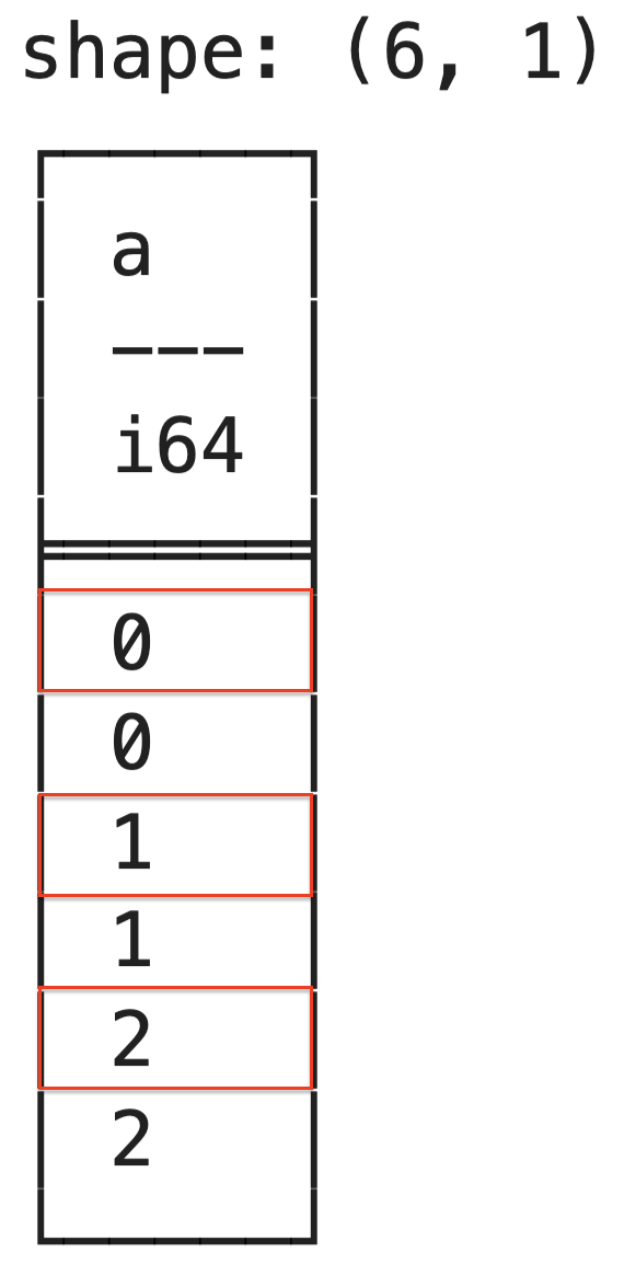
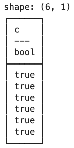
33이처럼 subset은 계산할 대상을 정의하는 하나이상의 열 표현식을 의미하며 데이터프레임 수준에서 작동합니다. 만약, 표현식 수준에서 하위 집합에 대해 작업하려면 struct를 사용하실 수 있습니다.
print(df.select(pl.struct("a", "b").n_unique()))print(df.select(pl.struct("a", "b").n_unique()))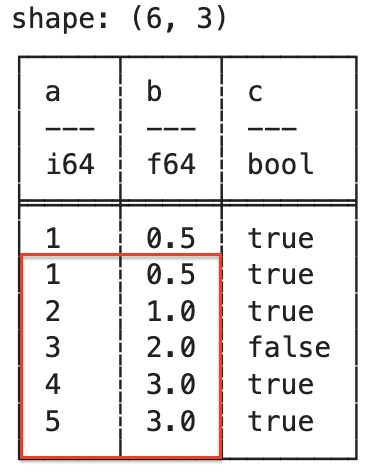
shape: (1, 1)
┌─────┐
│ a │
│ --- │
│ u32 │
╞═════╡
│ 5 │
└─────┘shape: (1, 1)
┌─────┐
│ a │
│ --- │
│ u32 │
╞═════╡
│ 5 │
└─────┘이 struct 방식은 표현식 내에서 사용하기 때문에 다른 표현식과 함께 메서드 체이닝을 사용하거나 복잡한 연산을 구성할 때 유연하게 사용할 수 있습니다.
- n_unique, subset : 단순히 고유값 개수만 필요할 때
- sturuct, n_unique : 복잡한 연산을 사용해야 할 때
열별 고유 값의 수를 계산하려는 경우 표현식 구문을 사용하여 해당 결과가 포함된 새 데이터프레임을 반환해보도록 하겠습니다. 출력 결과를 보시면 a열, b열의 고유값은 각각 1개 c열의 고유값은 2개가 있는 것을 확인하실 수 있습니다.
df = pl.DataFrame(
[[1, 2, 3], [1, 2, 4]], schema=["a", "b", "c"], orient="row"
)
df_nunique = df.select(pl.all().n_unique())
print(df_nunique)df = pl.DataFrame(
[[1, 2, 3], [1, 2, 4]], schema=["a", "b", "c"], orient="row"
)
df_nunique = df.select(pl.all().n_unique())
print(df_nunique)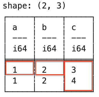
shape: (1, 3)
┌─────┬─────┬─────┐
│ a ┆ b ┆ c │
│ --- ┆ --- ┆ --- │
│ u32 ┆ u32 ┆ u32 │
╞═════╪═════╪═════╡
│ 1 ┆ 1 ┆ 2 │
└─────┴─────┴─────┘shape: (1, 3)
┌─────┬─────┬─────┐
│ a ┆ b ┆ c │
│ --- ┆ --- ┆ --- │
│ u32 ┆ u32 ┆ u32 │
╞═════╪═════╪═════╡
│ 1 ┆ 1 ┆ 2 │
└─────┴─────┴─────┘뒤에서 배울 내용이지만, group_by를 사용하여 그룹별 고유값을 반환할 수 있습니다.
df_agg_nunique = df.group_by("a").n_unique()
print(df_agg_nunique)df_agg_nunique = df.group_by("a").n_unique()
print(df_agg_nunique)shape: (1, 3)
┌─────┬─────┬─────┐
│ a ┆ b ┆ c │
│ --- ┆ --- ┆ --- │
│ i64 ┆ u32 ┆ u32 │
╞═════╪═════╪═════╡
│ 1 ┆ 1 ┆ 2 │
└─────┴─────┴─────┘shape: (1, 3)
┌─────┬─────┬─────┐
│ a ┆ b ┆ c │
│ --- ┆ --- ┆ --- │
│ i64 ┆ u32 ┆ u32 │
╞═════╪═════╪═════╡
│ 1 ┆ 1 ┆ 2 │
└─────┴─────┴─────┘8.6 is_empty
is_empty는 데이터프레임에 행이 없는 경우 True를 반환하고 행이 있으면 False를 반환합니다.
print(df.is_empty())print(df.is_empty())FalseFalsec열의 값이 10를 초과하는 값이 있는지 확인해보도록 하겠습니다. 출력 결과를 보시면 True로 출력되어 10이 초과하는 값이 없다는 것을 확인하실 수 있습니다.
print(df.filter(pl.col("c") > 10).is_empty())print(df.filter(pl.col("c") > 10).is_empty())TrueTrueis_emtpy 메서드를 지운 후에 실행시켜 보셔도 데이터프레임이 비어 있는 것을 확인하실 수 있습니다.
print(df.filter(pl.col("c") > 10))print(df.filter(pl.col("c") > 10))shape: (0, 3)
┌─────┬─────┬─────┐
│ a ┆ b ┆ c │
│ --- ┆ --- ┆ --- │
│ i64 ┆ i64 ┆ i64 │
╞═════╪═════╪═════╡
└─────┴─────┴─────┘shape: (0, 3)
┌─────┬─────┬─────┐
│ a ┆ b ┆ c │
│ --- ┆ --- ┆ --- │
│ i64 ┆ i64 ┆ i64 │
╞═════╪═════╪═════╡
└─────┴─────┴─────┘9. 데이터 정렬
9.1 sort
sort 메서드는 지정된 컬럼명을 기준으로 데이터프레임을 정렬합니다. 실습을 위해 데이터프레임을 생성하고 특정 컬럼을 기준으로 정렬합니다. a 열을 기준으로 오름차순으로 정렬해보도록 하겠습니다. 정렬 결과를 보면 null 이 가장 상단에 배치된 것을 보실 수 있습니다. 이는 polars에서 null이 가장 작은 값임을 의미합니다.
import polars as pl
df = pl.DataFrame(
{
"a": [1, 2, None],
"b": [6.0, 5.0, 4.0],
"c": ["a", "c", "b"],
}
)
# df.sort("컬럼명")
print(df.sort("a"))import polars as pl
df = pl.DataFrame(
{
"a": [1, 2, None],
"b": [6.0, 5.0, 4.0],
"c": ["a", "c", "b"],
}
)
# df.sort("컬럼명")
print(df.sort("a"))shape: (3, 3)
┌──────┬─────┬─────┐
│ a ┆ b ┆ c │
│ --- ┆ --- ┆ --- │
│ i64 ┆ f64 ┆ str │
╞══════╪═════╪═════╡
│ null ┆ 4.0 ┆ b │
│ 1 ┆ 6.0 ┆ a │
│ 2 ┆ 5.0 ┆ c │
└──────┴─────┴─────┘shape: (3, 3)
┌──────┬─────┬─────┐
│ a ┆ b ┆ c │
│ --- ┆ --- ┆ --- │
│ i64 ┆ f64 ┆ str │
╞══════╪═════╪═════╡
│ null ┆ 4.0 ┆ b │
│ 1 ┆ 6.0 ┆ a │
│ 2 ┆ 5.0 ┆ c │
└──────┴─────┴─────┘null의 크기 비교 처리 방식은 프로그래밍 언어와 라이브러리마다 다릅니다. 어떤 곳에서는 가장 큰 값으로 처리하고, 다른 곳에서는 가장 작은 값으로 처리합니다.
이번에는 계산식을 기준으로 정렬해보도록 하겠습니다. a열의 값과 b의 열의 값에 곱하기 2한 값을 더한 후에 이 값을 기준으로 오름차순으로 정렬하고 null 값은 마지막에 오도록 정렬해보도록 하겠습니다. 출력 결과를 보시면 계산식을 기준으로 정렬되었고 nulls_last를 True로 주어 null 값을 마지막에 오도록 설정하였습니다.
# df.sort("계산식")
print(df.sort(pl.col("a") + pl.col("b") * 2, nulls_last=True))# df.sort("계산식")
print(df.sort(pl.col("a") + pl.col("b") * 2, nulls_last=True))shape: (3, 3)
┌──────┬─────┬─────┐
│ a ┆ b ┆ c │
│ --- ┆ --- ┆ --- │
│ i64 ┆ f64 ┆ str │
╞══════╪═════╪═════╡
│ 2 ┆ 5.0 ┆ c │
│ 1 ┆ 6.0 ┆ a │
│ null ┆ 4.0 ┆ b │
└──────┴─────┴─────┘shape: (3, 3)
┌──────┬─────┬─────┐
│ a ┆ b ┆ c │
│ --- ┆ --- ┆ --- │
│ i64 ┆ f64 ┆ str │
╞══════╪═════╪═════╡
│ 2 ┆ 5.0 ┆ c │
│ 1 ┆ 6.0 ┆ a │
│ null ┆ 4.0 ┆ b │
└──────┴─────┴─────┘- nulls_last : 정렬할 때 null 값을 마지막에 오도록 지정할 수 있습니다.
nulls_last=True: 모든 열에 적용되는 단일 부울 값 지정nulls_last=[True, False, True]: 각 열에 대해 개별적으로 null 값 처리 방법을 부울 리스트 지정
이번에는 각 열에 대해 a, c 열만 nulls_last를 적용해보도록 하겠습니다.
print(df.sort([pl.col("a"), pl.col("b"), pl.col("c")], nulls_last=[True, False, True]))print(df.sort([pl.col("a"), pl.col("b"), pl.col("c")], nulls_last=[True, False, True]))shape: (3, 3)
┌──────┬─────┬─────┐
│ a ┆ b ┆ c │
│ --- ┆ --- ┆ --- │
│ i64 ┆ f64 ┆ str │
╞══════╪═════╪═════╡
│ 2 ┆ 5.0 ┆ c │
│ 1 ┆ 6.0 ┆ a │
│ null ┆ 4.0 ┆ b │
└──────┴─────┴─────┘shape: (3, 3)
┌──────┬─────┬─────┐
│ a ┆ b ┆ c │
│ --- ┆ --- ┆ --- │
│ i64 ┆ f64 ┆ str │
╞══════╪═════╪═════╡
│ 2 ┆ 5.0 ┆ c │
│ 1 ┆ 6.0 ┆ a │
│ null ┆ 4.0 ┆ b │
└──────┴─────┴─────┘이번에는 여러 컬럼명을 기준으로 내림차순으로 정렬해보도록 하겠습니다. 이때, 리스트에 정렬할 순서대로 컬럼명을 작성해주셔야 합니다. 출력 결과를 보시면 c열을 기준으로 먼저 내림차순 정렬하고 a열을 기준으로 내림차순 정렬된 것을 보실 수 있습니다.
print(df.sort(["c", "a"], descending=True))print(df.sort(["c", "a"], descending=True))- descending : 내림차순으로 정렬합니다.
shape: (3, 3)
┌──────┬─────┬─────┐
│ a ┆ b ┆ c │
│ --- ┆ --- ┆ --- │
│ i64 ┆ f64 ┆ str │
╞══════╪═════╪═════╡
│ 2 ┆ 5.0 ┆ c │
│ null ┆ 4.0 ┆ b │
│ 1 ┆ 6.0 ┆ a │
└──────┴─────┴─────┘shape: (3, 3)
┌──────┬─────┬─────┐
│ a ┆ b ┆ c │
│ --- ┆ --- ┆ --- │
│ i64 ┆ f64 ┆ str │
╞══════╪═════╪═════╡
│ 2 ┆ 5.0 ┆ c │
│ null ┆ 4.0 ┆ b │
│ 1 ┆ 6.0 ┆ a │
└──────┴─────┴─────┘descending는 nulls_last과 마찬가지로 여러 열을 기준으로 정렬하는 경우 부울 리스트 전달하여 열별로 지정할 수 있습니다. c열은 오름차순으로 정렬하고 a는 내림차순으로 정렬해보도록 하겠습니다.
print(df.sort(["c", "a"], descending=[False, True]))print(df.sort(["c", "a"], descending=[False, True]))shape: (3, 3)
┌──────┬─────┬─────┐
│ a ┆ b ┆ c │
│ --- ┆ --- ┆ --- │
│ i64 ┆ f64 ┆ str │
╞══════╪═════╪═════╡
│ 1 ┆ 6.0 ┆ a │
│ null ┆ 4.0 ┆ b │
│ 2 ┆ 5.0 ┆ c │
└──────┴─────┴─────┘shape: (3, 3)
┌──────┬─────┬─────┐
│ a ┆ b ┆ c │
│ --- ┆ --- ┆ --- │
│ i64 ┆ f64 ┆ str │
╞══════╪═════╪═════╡
│ 1 ┆ 6.0 ┆ a │
│ null ┆ 4.0 ┆ b │
│ 2 ┆ 5.0 ┆ c │
└──────┴─────┴─────┘쉼표로 컬럼명을 작성하셔도 여러 열을 기준으로 정렬할 수 있습니다.
df.sort("c", "a", descending=[False, True])df.sort("c", "a", descending=[False, True])shape: (3, 3)
┌──────┬─────┬─────┐
│ a ┆ b ┆ c │
│ --- ┆ --- ┆ --- │
│ i64 ┆ f64 ┆ str │
╞══════╪═════╪═════╡
│ 1 ┆ 6.0 ┆ a │
│ null ┆ 4.0 ┆ b │
│ 2 ┆ 5.0 ┆ c │
└──────┴─────┴─────┘shape: (3, 3)
┌──────┬─────┬─────┐
│ a ┆ b ┆ c │
│ --- ┆ --- ┆ --- │
│ i64 ┆ f64 ┆ str │
╞══════╪═════╪═════╡
│ 1 ┆ 6.0 ┆ a │
│ null ┆ 4.0 ┆ b │
│ 2 ┆ 5.0 ┆ c │
└──────┴─────┴─────┘요소가 동일한 경우 순서를 유지하고 싶다면 maintain_order 매개변수를 True로 설정합니다. c열을 기준으로 내림차순 정렬하고 데이터프레임 생성 순서와 동일하게 출력해보도록 하겠습니다. 출력 결과를 보시면 c열의 b의 값이 동일한 경우가 있는데 생성 순서대로 출력된 것을 보실 수 있습니다.
import polars as pl
df = pl.DataFrame(
{
"a": [1, 2, None],
"b": [6.0, 5.0, 5.0],
"c": ["a", "b", "b"],
}
)
print(df.sort("c", descending=True, maintain_order=True))import polars as pl
df = pl.DataFrame(
{
"a": [1, 2, None],
"b": [6.0, 5.0, 5.0],
"c": ["a", "b", "b"],
}
)
print(df.sort("c", descending=True, maintain_order=True))shape: (3, 3)
┌──────┬─────┬─────┐
│ a ┆ b ┆ c │
│ --- ┆ --- ┆ --- │
│ i64 ┆ f64 ┆ str │
╞══════╪═════╪═════╡
│ 2 ┆ 5.0 ┆ b │
│ null ┆ 5.0 ┆ b │
│ 1 ┆ 6.0 ┆ a │
└──────┴─────┴─────┘shape: (3, 3)
┌──────┬─────┬─────┐
│ a ┆ b ┆ c │
│ --- ┆ --- ┆ --- │
│ i64 ┆ f64 ┆ str │
╞══════╪═════╪═════╡
│ 2 ┆ 5.0 ┆ b │
│ null ┆ 5.0 ┆ b │
│ 1 ┆ 6.0 ┆ a │
└──────┴─────┴─────┘multithreaded 매개변수를 True(기본값)로 설정하여 데이터 정렬 시 여러 스레드를 사용하여 병렬 처리하여 성능을 최적화 할 수 있습니다.
print(df.sort("c", descending=True, multithreaded=True))print(df.sort("c", descending=True, multithreaded=True))multithreaded 옵션은 언제 사용하는가?
- 데이터셋이 매우 클 때
- 멀티코어 프로세서를 가지고 있을 때
- 데이터 정렬 작업이 시간이 많이 걸리는 경우 병렬 처리 혜택을 원할 때
작은 데이터 셋이나 디버깅을 쉽게 하고 싶은 경우에는 멀티 스레드를 사용하면 스레드를 생성하고 관리하는 오버헤드가 실제 정렬 시간보다 더 오래 걸릴 수 있습니다. 이럴 때는 단일 스레드를 사용하는 것이 더 효율적일 수 있습니다.
9.2 reverse
데이터프레임을 반대로 뒤집습니다. 출력 결과를 보시면 데이터가 가장 늦게 생성된 행 부터 출력되는 것을 보실 수 있습니다.
df = pl.DataFrame(
{
"key": ["a", "b", "c"],
"val": [1, 2, 3],
}
)
print(df.reverse())df = pl.DataFrame(
{
"key": ["a", "b", "c"],
"val": [1, 2, 3],
}
)
print(df.reverse())shape: (3, 2)
┌─────┬─────┐
│ key ┆ val │
│ --- ┆ --- │
│ str ┆ i64 │
╞═════╪═════╡
│ c ┆ 3 │
│ b ┆ 2 │
│ a ┆ 1 │
└─────┴─────┘shape: (3, 2)
┌─────┬─────┐
│ key ┆ val │
│ --- ┆ --- │
│ str ┆ i64 │
╞═════╪═════╡
│ c ┆ 3 │
│ b ┆ 2 │
│ a ┆ 1 │
└─────┴─────┘10. 문자열 처리 방법
먼저, 실습을 위해 데이터프레임을 생성하도록 하겠습니다.
df = pl.DataFrame({
"station": ["Station " + str(x) for x in range(1, 6)],
"temperatures": [
"20 5 5 E1 7 13 19 9 6 20",
"18 8 16 11 23 E2 8 E2 E2 E2 90 70 40",
"19 24 E9 16 6 12 10 22",
"E2 E0 15 7 8 10 E1 24 17 13 6",
"14 8 E0 16 22 24 E1",
],
"text": [
" Hello World ",
" Python Data***",
"***Analysis ",
"Polars Lib ",
" DataFrame"
]
})
print(df)df = pl.DataFrame({
"station": ["Station " + str(x) for x in range(1, 6)],
"temperatures": [
"20 5 5 E1 7 13 19 9 6 20",
"18 8 16 11 23 E2 8 E2 E2 E2 90 70 40",
"19 24 E9 16 6 12 10 22",
"E2 E0 15 7 8 10 E1 24 17 13 6",
"14 8 E0 16 22 24 E1",
],
"text": [
" Hello World ",
" Python Data***",
"***Analysis ",
"Polars Lib ",
" DataFrame"
]
})
print(df)shape: (5, 3)
┌───────────┬─────────────────────────────────┬───────────────────┐
│ station ┆ temperatures ┆ text │
│ --- ┆ --- ┆ --- │
│ str ┆ str ┆ str │
╞═══════════╪═════════════════════════════════╪═══════════════════╡
│ Station 1 ┆ 20 5 5 E1 7 13 19 9 6 20 ┆ Hello World │
│ Station 2 ┆ 18 8 16 11 23 E2 8 E2 E2 E2 90… ┆ Python Data*** │
│ Station 3 ┆ 19 24 E9 16 6 12 10 22 ┆ ***Analysis │
│ Station 4 ┆ E2 E0 15 7 8 10 E1 24 17 13 6 ┆ Polars Lib │
│ Station 5 ┆ 14 8 E0 16 22 24 E1 ┆ DataFrame │
└───────────┴─────────────────────────────────┴───────────────────┘shape: (5, 3)
┌───────────┬─────────────────────────────────┬───────────────────┐
│ station ┆ temperatures ┆ text │
│ --- ┆ --- ┆ --- │
│ str ┆ str ┆ str │
╞═══════════╪═════════════════════════════════╪═══════════════════╡
│ Station 1 ┆ 20 5 5 E1 7 13 19 9 6 20 ┆ Hello World │
│ Station 2 ┆ 18 8 16 11 23 E2 8 E2 E2 E2 90… ┆ Python Data*** │
│ Station 3 ┆ 19 24 E9 16 6 12 10 22 ┆ ***Analysis │
│ Station 4 ┆ E2 E0 15 7 8 10 E1 24 17 13 6 ┆ Polars Lib │
│ Station 5 ┆ 14 8 E0 16 22 24 E1 ┆ DataFrame │
└───────────┴─────────────────────────────────┴───────────────────┘데이터프레임의 temperatures 열의 타입을 확인해보시면 문자열인 것을 보실 수 있습니다.
print(df['temperatures'].dtype)print(df['temperatures'].dtype)StringString10. 문자열 처리 방법
먼저, 실습을 위해 데이터프레임을 생성하도록 하겠습니다.
df = pl.DataFrame({
"station": ["Station " + str(x) for x in range(1, 6)],
"temperatures": [
"20 5 5 E1 7 13 19 9 6 20",
"18 8 16 11 23 E2 8 E2 E2 E2 90 70 40",
"19 24 E9 16 6 12 10 22",
"E2 E0 15 7 8 10 E1 24 17 13 6",
"14 8 E0 16 22 24 E1",
],
"text": [
" Hello World ",
" Python Data***",
"***Analysis ",
"Polars Lib ",
" DataFrame"
]
})
print(df)df = pl.DataFrame({
"station": ["Station " + str(x) for x in range(1, 6)],
"temperatures": [
"20 5 5 E1 7 13 19 9 6 20",
"18 8 16 11 23 E2 8 E2 E2 E2 90 70 40",
"19 24 E9 16 6 12 10 22",
"E2 E0 15 7 8 10 E1 24 17 13 6",
"14 8 E0 16 22 24 E1",
],
"text": [
" Hello World ",
" Python Data***",
"***Analysis ",
"Polars Lib ",
" DataFrame"
]
})
print(df)shape: (5, 3)
┌───────────┬─────────────────────────────────┬───────────────────┐
│ station ┆ temperatures ┆ text │
│ --- ┆ --- ┆ --- │
│ str ┆ str ┆ str │
╞═══════════╪═════════════════════════════════╪═══════════════════╡
│ Station 1 ┆ 20 5 5 E1 7 13 19 9 6 20 ┆ Hello World │
│ Station 2 ┆ 18 8 16 11 23 E2 8 E2 E2 E2 90… ┆ Python Data*** │
│ Station 3 ┆ 19 24 E9 16 6 12 10 22 ┆ ***Analysis │
│ Station 4 ┆ E2 E0 15 7 8 10 E1 24 17 13 6 ┆ Polars Lib │
│ Station 5 ┆ 14 8 E0 16 22 24 E1 ┆ DataFrame │
└───────────┴─────────────────────────────────┴───────────────────┘shape: (5, 3)
┌───────────┬─────────────────────────────────┬───────────────────┐
│ station ┆ temperatures ┆ text │
│ --- ┆ --- ┆ --- │
│ str ┆ str ┆ str │
╞═══════════╪═════════════════════════════════╪═══════════════════╡
│ Station 1 ┆ 20 5 5 E1 7 13 19 9 6 20 ┆ Hello World │
│ Station 2 ┆ 18 8 16 11 23 E2 8 E2 E2 E2 90… ┆ Python Data*** │
│ Station 3 ┆ 19 24 E9 16 6 12 10 22 ┆ ***Analysis │
│ Station 4 ┆ E2 E0 15 7 8 10 E1 24 17 13 6 ┆ Polars Lib │
│ Station 5 ┆ 14 8 E0 16 22 24 E1 ┆ DataFrame │
└───────────┴─────────────────────────────────┴───────────────────┘데이터프레임의 temperatures 열의 타입을 확인해보시면 문자열인 것을 보실 수 있습니다.
print(df['temperatures'].dtype)print(df['temperatures'].dtype)StringString10.1 문자열 조작
10.1.1 문자열 길이
print(df.with_columns(pl.col("text").str.len_chars().alias("text_length")))print(df.with_columns(pl.col("text").str.len_chars().alias("text_length")))str.len_chars(): 문자열의 길이 반환합니다.
shape: (5, 4)
┌───────────┬─────────────────────────────────┬───────────────────┬─────────────┐
│ station ┆ temperatures ┆ text ┆ text_length │
│ --- ┆ --- ┆ --- ┆ --- │
│ str ┆ str ┆ str ┆ u32 │
╞═══════════╪═════════════════════════════════╪═══════════════════╪═════════════╡
│ Station 1 ┆ 20 5 5 E1 7 13 19 9 6 20 ┆ Hello World ┆ 17 │
│ Station 2 ┆ 18 8 16 11 23 E2 8 E2 E2 E2 90… ┆ Python Data*** ┆ 17 │
│ Station 3 ┆ 19 24 E9 16 6 12 10 22 ┆ ***Analysis ┆ 14 │
│ Station 4 ┆ E2 E0 15 7 8 10 E1 24 17 13 6 ┆ Polars Lib ┆ 13 │
│ Station 5 ┆ 14 8 E0 16 22 24 E1 ┆ DataFrame ┆ 12 │
└───────────┴─────────────────────────────────┴───────────────────┴─────────────┘shape: (5, 4)
┌───────────┬─────────────────────────────────┬───────────────────┬─────────────┐
│ station ┆ temperatures ┆ text ┆ text_length │
│ --- ┆ --- ┆ --- ┆ --- │
│ str ┆ str ┆ str ┆ u32 │
╞═══════════╪═════════════════════════════════╪═══════════════════╪═════════════╡
│ Station 1 ┆ 20 5 5 E1 7 13 19 9 6 20 ┆ Hello World ┆ 17 │
│ Station 2 ┆ 18 8 16 11 23 E2 8 E2 E2 E2 90… ┆ Python Data*** ┆ 17 │
│ Station 3 ┆ 19 24 E9 16 6 12 10 22 ┆ ***Analysis ┆ 14 │
│ Station 4 ┆ E2 E0 15 7 8 10 E1 24 17 13 6 ┆ Polars Lib ┆ 13 │
│ Station 5 ┆ 14 8 E0 16 22 24 E1 ┆ DataFrame ┆ 12 │
└───────────┴─────────────────────────────────┴───────────────────┴─────────────┘10.1.2 대소문자 변환
print(df.with_columns([
pl.col("text").str.to_uppercase().alias('text_upper'),
pl.col("text").str.to_lowercase().alias('text_lower')
]))print(df.with_columns([
pl.col("text").str.to_uppercase().alias('text_upper'),
pl.col("text").str.to_lowercase().alias('text_lower')
]))str.to_uppercase(): 모든 문자를 대문자로 변환합니다.str.to_lowercase(): 모든 문자를 소문자로 변환합니다.
shape: (5, 5)
┌───────────┬──────────────────────────┬───────────────────┬───────────────────┬───────────────────┐
│ station ┆ temperatures ┆ text ┆ text_upper ┆ text_lower │
│ --- ┆ --- ┆ --- ┆ --- ┆ --- │
│ str ┆ str ┆ str ┆ str ┆ str │
╞═══════════╪══════════════════════════╪═══════════════════╪═══════════════════╪═══════════════════╡
│ Station 1 ┆ 20 5 5 E1 7 13 19 9 6 20 ┆ Hello World ┆ HELLO WORLD ┆ hello world │
│ Station 2 ┆ 18 8 16 11 23 E2 8 E2 E2 ┆ Python Data*** ┆ PYTHON DATA*** ┆ python data*** │
│ ┆ E2 90… ┆ ┆ ┆ │
│ Station 3 ┆ 19 24 E9 16 6 12 10 22 ┆ ***Analysis ┆ ***ANALYSIS ┆ ***analysis │
│ Station 4 ┆ E2 E0 15 7 8 10 E1 24 17 ┆ Polars Lib ┆ POLARS LIB ┆ polars lib │
│ ┆ 13 6 ┆ ┆ ┆ │
│ Station 5 ┆ 14 8 E0 16 22 24 E1 ┆ DataFrame ┆ DATAFRAME ┆ dataframe │
└───────────┴──────────────────────────┴───────────────────┴───────────────────┴───────────────────┘shape: (5, 5)
┌───────────┬──────────────────────────┬───────────────────┬───────────────────┬───────────────────┐
│ station ┆ temperatures ┆ text ┆ text_upper ┆ text_lower │
│ --- ┆ --- ┆ --- ┆ --- ┆ --- │
│ str ┆ str ┆ str ┆ str ┆ str │
╞═══════════╪══════════════════════════╪═══════════════════╪═══════════════════╪═══════════════════╡
│ Station 1 ┆ 20 5 5 E1 7 13 19 9 6 20 ┆ Hello World ┆ HELLO WORLD ┆ hello world │
│ Station 2 ┆ 18 8 16 11 23 E2 8 E2 E2 ┆ Python Data*** ┆ PYTHON DATA*** ┆ python data*** │
│ ┆ E2 90… ┆ ┆ ┆ │
│ Station 3 ┆ 19 24 E9 16 6 12 10 22 ┆ ***Analysis ┆ ***ANALYSIS ┆ ***analysis │
│ Station 4 ┆ E2 E0 15 7 8 10 E1 24 17 ┆ Polars Lib ┆ POLARS LIB ┆ polars lib │
│ ┆ 13 6 ┆ ┆ ┆ │
│ Station 5 ┆ 14 8 E0 16 22 24 E1 ┆ DataFrame ┆ DATAFRAME ┆ dataframe │
└───────────┴──────────────────────────┴───────────────────┴───────────────────┴───────────────────┘10.1.3 특정 구분자 제거
print(df.with_columns([
pl.col("text").str.strip_chars(" ").alias("strip_all"),
pl.col("text").str.strip_chars_start("*").alias("strip_left"),
pl.col("text").str.strip_chars_end("*").alias("strip_right")
]))print(df.with_columns([
pl.col("text").str.strip_chars(" ").alias("strip_all"),
pl.col("text").str.strip_chars_start("*").alias("strip_left"),
pl.col("text").str.strip_chars_end("*").alias("strip_right")
]))str.strip_chars('구분자'): 양쪽에 있는 구분자 제거합니다.str.strip_chars_start('구분자'): 왼쪽에 있는 구분자 제거합니다.str.strip_chars_end('구분자'): 오른쪽에 있는 구분자 제거합니다.
shape: (5, 6)
┌───────────┬─────────────────┬─────────────────┬────────────────┬────────────────┬────────────────┐
│ station ┆ temperatures ┆ text ┆ strip_all ┆ strip_left ┆ strip_right │
│ --- ┆ --- ┆ --- ┆ --- ┆ --- ┆ --- │
│ str ┆ str ┆ str ┆ str ┆ str ┆ str │
╞═══════════╪═════════════════╪═════════════════╪════════════════╪════════════════╪════════════════╡
│ Station 1 ┆ 20 5 5 E1 7 13 ┆ Hello World ┆ Hello World ┆ Hello World ┆ Hello World │
│ ┆ 19 9 6 20 ┆ ┆ ┆ ┆ │
│ Station 2 ┆ 18 8 16 11 23 ┆ Python Data*** ┆ Python Data*** ┆ Python Data*** ┆ Python Data │
│ ┆ E2 8 E2 E2 E2 ┆ ┆ ┆ ┆ │
│ ┆ 90… ┆ ┆ ┆ ┆ │
│ Station 3 ┆ 19 24 E9 16 6 ┆ ***Analysis ┆ ***Analysis ┆ Analysis ┆ ***Analysis │
│ ┆ 12 10 22 ┆ ┆ ┆ ┆ │
│ Station 4 ┆ E2 E0 15 7 8 10 ┆ Polars Lib ┆ Polars Lib ┆ Polars Lib ┆ Polars Lib │
│ ┆ E1 24 17 13 6 ┆ ┆ ┆ ┆ │
│ Station 5 ┆ 14 8 E0 16 22 ┆ DataFrame ┆ DataFrame ┆ DataFrame ┆ DataFrame │
│ ┆ 24 E1 ┆ ┆ ┆ ┆ │
└───────────┴─────────────────┴─────────────────┴────────────────┴────────────────┴────────────────┘shape: (5, 6)
┌───────────┬─────────────────┬─────────────────┬────────────────┬────────────────┬────────────────┐
│ station ┆ temperatures ┆ text ┆ strip_all ┆ strip_left ┆ strip_right │
│ --- ┆ --- ┆ --- ┆ --- ┆ --- ┆ --- │
│ str ┆ str ┆ str ┆ str ┆ str ┆ str │
╞═══════════╪═════════════════╪═════════════════╪════════════════╪════════════════╪════════════════╡
│ Station 1 ┆ 20 5 5 E1 7 13 ┆ Hello World ┆ Hello World ┆ Hello World ┆ Hello World │
│ ┆ 19 9 6 20 ┆ ┆ ┆ ┆ │
│ Station 2 ┆ 18 8 16 11 23 ┆ Python Data*** ┆ Python Data*** ┆ Python Data*** ┆ Python Data │
│ ┆ E2 8 E2 E2 E2 ┆ ┆ ┆ ┆ │
│ ┆ 90… ┆ ┆ ┆ ┆ │
│ Station 3 ┆ 19 24 E9 16 6 ┆ ***Analysis ┆ ***Analysis ┆ Analysis ┆ ***Analysis │
│ ┆ 12 10 22 ┆ ┆ ┆ ┆ │
│ Station 4 ┆ E2 E0 15 7 8 10 ┆ Polars Lib ┆ Polars Lib ┆ Polars Lib ┆ Polars Lib │
│ ┆ E1 24 17 13 6 ┆ ┆ ┆ ┆ │
│ Station 5 ┆ 14 8 E0 16 22 ┆ DataFrame ┆ DataFrame ┆ DataFrame ┆ DataFrame │
│ ┆ 24 E1 ┆ ┆ ┆ ┆ │
└───────────┴─────────────────┴─────────────────┴────────────────┴────────────────┴────────────────┘10.1.4 지정 문자 채우기
print(df.with_columns([
# 15자리가 되도록 앞쪽에 '*' 추가
pl.col("text").str.pad_start(15, '*').alias("padded_start"),
# 15자리가 되도록 뒤쪽에 '#' 추가
pl.col("text").str.pad_end(15, '#').alias("padded_end")
]))print(df.with_columns([
# 15자리가 되도록 앞쪽에 '*' 추가
pl.col("text").str.pad_start(15, '*').alias("padded_start"),
# 15자리가 되도록 뒤쪽에 '#' 추가
pl.col("text").str.pad_end(15, '#').alias("padded_end")
]))str.pad_start(문자열 길이, ‘문자’): 문자열 길이를 지정하고 앞쪽을 지정한 문자로 채웁니다.str.pad_end(문자열 길이, ‘문자’): 문자열 길이를 지정하고 문자열 뒤쪽을 지정한 문자로 채웁니다.
shape: (5, 5)
┌───────────┬──────────────────────────┬───────────────────┬───────────────────┬───────────────────┐
│ station ┆ temperatures ┆ text ┆ padded_start ┆ padded_end │
│ --- ┆ --- ┆ --- ┆ --- ┆ --- │
│ str ┆ str ┆ str ┆ str ┆ str │
╞═══════════╪══════════════════════════╪═══════════════════╪═══════════════════╪═══════════════════╡
│ Station 1 ┆ 20 5 5 E1 7 13 19 9 6 20 ┆ Hello World ┆ Hello World ┆ Hello World │
│ Station 2 ┆ 18 8 16 11 23 E2 8 E2 E2 ┆ Python Data*** ┆ Python Data*** ┆ Python Data*** │
│ ┆ E2 90… ┆ ┆ ┆ │
│ Station 3 ┆ 19 24 E9 16 6 12 10 22 ┆ ***Analysis ┆ ****Analysis ┆ ***Analysis # │
│ Station 4 ┆ E2 E0 15 7 8 10 E1 24 17 ┆ Polars Lib ┆ **Polars Lib ┆ Polars Lib ## │
│ ┆ 13 6 ┆ ┆ ┆ │
│ Station 5 ┆ 14 8 E0 16 22 24 E1 ┆ DataFrame ┆ *** DataFrame ┆ DataFrame### │
└───────────┴──────────────────────────┴───────────────────┴───────────────────┴───────────────────┘shape: (5, 5)
┌───────────┬──────────────────────────┬───────────────────┬───────────────────┬───────────────────┐
│ station ┆ temperatures ┆ text ┆ padded_start ┆ padded_end │
│ --- ┆ --- ┆ --- ┆ --- ┆ --- │
│ str ┆ str ┆ str ┆ str ┆ str │
╞═══════════╪══════════════════════════╪═══════════════════╪═══════════════════╪═══════════════════╡
│ Station 1 ┆ 20 5 5 E1 7 13 19 9 6 20 ┆ Hello World ┆ Hello World ┆ Hello World │
│ Station 2 ┆ 18 8 16 11 23 E2 8 E2 E2 ┆ Python Data*** ┆ Python Data*** ┆ Python Data*** │
│ ┆ E2 90… ┆ ┆ ┆ │
│ Station 3 ┆ 19 24 E9 16 6 12 10 22 ┆ ***Analysis ┆ ****Analysis ┆ ***Analysis # │
│ Station 4 ┆ E2 E0 15 7 8 10 E1 24 17 ┆ Polars Lib ┆ **Polars Lib ┆ Polars Lib ## │
│ ┆ 13 6 ┆ ┆ ┆ │
│ Station 5 ┆ 14 8 E0 16 22 24 E1 ┆ DataFrame ┆ *** DataFrame ┆ DataFrame### │
└───────────┴──────────────────────────┴───────────────────┴───────────────────┴───────────────────┘10.2 문자열 검색 및 치환
10.2.1 문자열 치환
temperatures 열의 모든 'E'를 'W'로 대체해보도록 하겠습니다.
# pl.col(columns).str.replace('바꿀값', '대체할 문자열')
print(df.with_columns(
pl.col("temperatures").str.replace("E","W")
))# pl.col(columns).str.replace('바꿀값', '대체할 문자열')
print(df.with_columns(
pl.col("temperatures").str.replace("E","W")
))str.replace('바꿀값', '대체할 문자열'): 문자열 내의 특정 부분을 다른 문자열로 대체할 수 있습니다.
shape: (5, 3)
┌───────────┬─────────────────────────────────┬───────────────────┐
│ station ┆ temperatures ┆ text │
│ --- ┆ --- ┆ --- │
│ str ┆ str ┆ str │
╞═══════════╪═════════════════════════════════╪═══════════════════╡
│ Station 1 ┆ 20 5 5 W1 7 13 19 9 6 20 ┆ Hello World │
│ Station 2 ┆ 18 8 16 11 23 W2 8 E2 E2 E2 90… ┆ Python Data*** │
│ Station 3 ┆ 19 24 W9 16 6 12 10 22 ┆ ***Analysis │
│ Station 4 ┆ W2 E0 15 7 8 10 E1 24 17 13 6 ┆ Polars Lib │
│ Station 5 ┆ 14 8 W0 16 22 24 E1 ┆ DataFrame │
└───────────┴─────────────────────────────────┴───────────────────┘shape: (5, 3)
┌───────────┬─────────────────────────────────┬───────────────────┐
│ station ┆ temperatures ┆ text │
│ --- ┆ --- ┆ --- │
│ str ┆ str ┆ str │
╞═══════════╪═════════════════════════════════╪═══════════════════╡
│ Station 1 ┆ 20 5 5 W1 7 13 19 9 6 20 ┆ Hello World │
│ Station 2 ┆ 18 8 16 11 23 W2 8 E2 E2 E2 90… ┆ Python Data*** │
│ Station 3 ┆ 19 24 W9 16 6 12 10 22 ┆ ***Analysis │
│ Station 4 ┆ W2 E0 15 7 8 10 E1 24 17 13 6 ┆ Polars Lib │
│ Station 5 ┆ 14 8 W0 16 22 24 E1 ┆ DataFrame │
└───────────┴─────────────────────────────────┴───────────────────┘pl.col()을 사용하지 않고 데이터프레임[’컬럼명’]으로 접근하여 문자열을 대체할 수도 있습니다.
# df.columns.str.replace('바꿀값', '대체할 문자열')
print(df.with_columns(
df['temperatures'].str.replace("E","W")
))# df.columns.str.replace('바꿀값', '대체할 문자열')
print(df.with_columns(
df['temperatures'].str.replace("E","W")
))shape: (5, 3)
┌───────────┬─────────────────────────────────┬───────────────────┐
│ station ┆ temperatures ┆ text │
│ --- ┆ --- ┆ --- │
│ str ┆ str ┆ str │
╞═══════════╪═════════════════════════════════╪═══════════════════╡
│ Station 1 ┆ 20 5 5 W1 7 13 19 9 6 20 ┆ Hello World │
│ Station 2 ┆ 18 8 16 11 23 W2 8 E2 E2 E2 90… ┆ Python Data*** │
│ Station 3 ┆ 19 24 W9 16 6 12 10 22 ┆ ***Analysis │
│ Station 4 ┆ W2 E0 15 7 8 10 E1 24 17 13 6 ┆ Polars Lib │
│ Station 5 ┆ 14 8 W0 16 22 24 E1 ┆ DataFrame │
└───────────┴─────────────────────────────────┴───────────────────┘shape: (5, 3)
┌───────────┬─────────────────────────────────┬───────────────────┐
│ station ┆ temperatures ┆ text │
│ --- ┆ --- ┆ --- │
│ str ┆ str ┆ str │
╞═══════════╪═════════════════════════════════╪═══════════════════╡
│ Station 1 ┆ 20 5 5 W1 7 13 19 9 6 20 ┆ Hello World │
│ Station 2 ┆ 18 8 16 11 23 W2 8 E2 E2 E2 90… ┆ Python Data*** │
│ Station 3 ┆ 19 24 W9 16 6 12 10 22 ┆ ***Analysis │
│ Station 4 ┆ W2 E0 15 7 8 10 E1 24 17 13 6 ┆ Polars Lib │
│ Station 5 ┆ 14 8 W0 16 22 24 E1 ┆ DataFrame │
└───────────┴─────────────────────────────────┴───────────────────┘위의 코드 실행결과를 보시면 첫번째로 나온 문자 E 만 W 로 바뀐것을 보실 수 있는데요. 만약, 모든 E 문자를 W로 바꾸고 싶으시다면 str.replace_all('바꿀값', '대체할 문자열') 메서드를 사용하셔야 합니다.
print(df.with_columns(
df['temperatures'].str.replace_all("E","W")
))print(df.with_columns(
df['temperatures'].str.replace_all("E","W")
))shape: (5, 3)
┌───────────┬─────────────────────────────────┬───────────────────┐
│ station ┆ temperatures ┆ text │
│ --- ┆ --- ┆ --- │
│ str ┆ str ┆ str │
╞═══════════╪═════════════════════════════════╪═══════════════════╡
│ Station 1 ┆ 20 5 5 W1 7 13 19 9 6 20 ┆ Hello World │
│ Station 2 ┆ 18 8 16 11 23 W2 8 W2 W2 W2 90… ┆ Python Data*** │
│ Station 3 ┆ 19 24 W9 16 6 12 10 22 ┆ ***Analysis │
│ Station 4 ┆ W2 W0 15 7 8 10 W1 24 17 13 6 ┆ Polars Lib │
│ Station 5 ┆ 14 8 W0 16 22 24 W1 ┆ DataFrame │
└───────────┴─────────────────────────────────┴───────────────────┘shape: (5, 3)
┌───────────┬─────────────────────────────────┬───────────────────┐
│ station ┆ temperatures ┆ text │
│ --- ┆ --- ┆ --- │
│ str ┆ str ┆ str │
╞═══════════╪═════════════════════════════════╪═══════════════════╡
│ Station 1 ┆ 20 5 5 W1 7 13 19 9 6 20 ┆ Hello World │
│ Station 2 ┆ 18 8 16 11 23 W2 8 W2 W2 W2 90… ┆ Python Data*** │
│ Station 3 ┆ 19 24 W9 16 6 12 10 22 ┆ ***Analysis │
│ Station 4 ┆ W2 W0 15 7 8 10 W1 24 17 13 6 ┆ Polars Lib │
│ Station 5 ┆ 14 8 W0 16 22 24 W1 ┆ DataFrame │
└───────────┴─────────────────────────────────┴───────────────────┘만약 한번에 여러 문자열을 다른 문자열로 대체하고 싶으시다면 str.replace_many('바꿀값', '대체할 문자열') 메서드를 사용하셔야 합니다.
text 열의 공백과 별표(*)를 삭제해보도록 하겠습니다.
print(df.with_columns(
df['text'].str.replace_many([' ','*'],'')
))print(df.with_columns(
df['text'].str.replace_many([' ','*'],'')
))shape: (5, 3)
┌───────────┬─────────────────────────────────┬─────────────┐
│ station ┆ temperatures ┆ text │
│ --- ┆ --- ┆ --- │
│ str ┆ str ┆ str │
╞═══════════╪═════════════════════════════════╪═════════════╡
│ Station 1 ┆ 20 5 5 E1 7 13 19 9 6 20 ┆ Hello World │
│ Station 2 ┆ 18 8 16 11 23 E2 8 E2 E2 E2 90… ┆ Python Data │
│ Station 3 ┆ 19 24 E9 16 6 12 10 22 ┆ Analysis │
│ Station 4 ┆ E2 E0 15 7 8 10 E1 24 17 13 6 ┆ Polars Lib │
│ Station 5 ┆ 14 8 E0 16 22 24 E1 ┆ DataFrame │
└───────────┴─────────────────────────────────┴─────────────┘shape: (5, 3)
┌───────────┬─────────────────────────────────┬─────────────┐
│ station ┆ temperatures ┆ text │
│ --- ┆ --- ┆ --- │
│ str ┆ str ┆ str │
╞═══════════╪═════════════════════════════════╪═════════════╡
│ Station 1 ┆ 20 5 5 E1 7 13 19 9 6 20 ┆ Hello World │
│ Station 2 ┆ 18 8 16 11 23 E2 8 E2 E2 E2 90… ┆ Python Data │
│ Station 3 ┆ 19 24 E9 16 6 12 10 22 ┆ Analysis │
│ Station 4 ┆ E2 E0 15 7 8 10 E1 24 17 13 6 ┆ Polars Lib │
│ Station 5 ┆ 14 8 E0 16 22 24 E1 ┆ DataFrame │
└───────────┴─────────────────────────────────┴─────────────┘이번에는 Python을 Java로 Polars를 Pandas로 대체해보도록 하겠습니다.
print(df.with_columns(
df['text'].str.replace_many(['Python','Polars'],['Java','Pandas'])
))print(df.with_columns(
df['text'].str.replace_many(['Python','Polars'],['Java','Pandas'])
))shape: (5, 3)
┌───────────┬─────────────────────────────────┬───────────────────┐
│ station ┆ temperatures ┆ text │
│ --- ┆ --- ┆ --- │
│ str ┆ str ┆ str │
╞═══════════╪═════════════════════════════════╪═══════════════════╡
│ Station 1 ┆ 20 5 5 E1 7 13 19 9 6 20 ┆ Hello World │
│ Station 2 ┆ 18 8 16 11 23 E2 8 E2 E2 E2 90… ┆ Java Data*** │
│ Station 3 ┆ 19 24 E9 16 6 12 10 22 ┆ ***Analysis │
│ Station 4 ┆ E2 E0 15 7 8 10 E1 24 17 13 6 ┆ Pandas Lib │
│ Station 5 ┆ 14 8 E0 16 22 24 E1 ┆ DataFrame │
└───────────┴─────────────────────────────────┴───────────────────┘shape: (5, 3)
┌───────────┬─────────────────────────────────┬───────────────────┐
│ station ┆ temperatures ┆ text │
│ --- ┆ --- ┆ --- │
│ str ┆ str ┆ str │
╞═══════════╪═════════════════════════════════╪═══════════════════╡
│ Station 1 ┆ 20 5 5 E1 7 13 19 9 6 20 ┆ Hello World │
│ Station 2 ┆ 18 8 16 11 23 E2 8 E2 E2 E2 90… ┆ Java Data*** │
│ Station 3 ┆ 19 24 E9 16 6 12 10 22 ┆ ***Analysis │
│ Station 4 ┆ E2 E0 15 7 8 10 E1 24 17 13 6 ┆ Pandas Lib │
│ Station 5 ┆ 14 8 E0 16 22 24 E1 ┆ DataFrame │
└───────────┴─────────────────────────────────┴───────────────────┘이처럼 여러개의 문자열을 다른 문자열로 대체할 때 Pandas에서는 메서드 체이닝을 사용하여 replace 메서드를 여러번 사용해야하지만 Polars는 replace_many 메서드를 통해 한번에 문자열을 대체할 수 있습니다.
10.2.2 특정 위치 문자열 확인
info = pl.DataFrame({
"email": [
"user@gmail.com",
"test@yahoo.com",
"admin@gmail.com",
"info@naver.com",
"contact@gmail.com"
],
"filename": [
"report.pdf",
"data.csv",
"image.jpg",
"document.pdf",
"sheet.xlsx"
]
})
print(info.with_columns([
# 1. 이메일이 'user'로 시작하는지 확인
pl.col("email").str.starts_with("user").alias("starts_with_user"),
# 2. 파일이 특정 확장자로 끝나는지 확인
pl.col("filename").str.ends_with(".csv").alias("is_csv")
]))info = pl.DataFrame({
"email": [
"user@gmail.com",
"test@yahoo.com",
"admin@gmail.com",
"info@naver.com",
"contact@gmail.com"
],
"filename": [
"report.pdf",
"data.csv",
"image.jpg",
"document.pdf",
"sheet.xlsx"
]
})
print(info.with_columns([
# 1. 이메일이 'user'로 시작하는지 확인
pl.col("email").str.starts_with("user").alias("starts_with_user"),
# 2. 파일이 특정 확장자로 끝나는지 확인
pl.col("filename").str.ends_with(".csv").alias("is_csv")
]))str.starts_with('문자열'): 특정 문자열로 시작하는지 확인합니다.str.ends_with('문자열'): 특정 문자열로 끝나는지 확인합니다.
shape: (5, 4)
┌───────────────────┬──────────────┬──────────────────┬────────┐
│ email ┆ filename ┆ starts_with_user ┆ is_csv │
│ --- ┆ --- ┆ --- ┆ --- │
│ str ┆ str ┆ bool ┆ bool │
╞═══════════════════╪══════════════╪══════════════════╪════════╡
│ user@gmail.com ┆ report.pdf ┆ true ┆ false │
│ test@yahoo.com ┆ data.csv ┆ false ┆ true │
│ admin@gmail.com ┆ image.jpg ┆ false ┆ false │
│ info@naver.com ┆ document.pdf ┆ false ┆ false │
│ contact@gmail.com ┆ sheet.xlsx ┆ false ┆ false │
└───────────────────┴──────────────┴──────────────────┴────────┘shape: (5, 4)
┌───────────────────┬──────────────┬──────────────────┬────────┐
│ email ┆ filename ┆ starts_with_user ┆ is_csv │
│ --- ┆ --- ┆ --- ┆ --- │
│ str ┆ str ┆ bool ┆ bool │
╞═══════════════════╪══════════════╪══════════════════╪════════╡
│ user@gmail.com ┆ report.pdf ┆ true ┆ false │
│ test@yahoo.com ┆ data.csv ┆ false ┆ true │
│ admin@gmail.com ┆ image.jpg ┆ false ┆ false │
│ info@naver.com ┆ document.pdf ┆ false ┆ false │
│ contact@gmail.com ┆ sheet.xlsx ┆ false ┆ false │
└───────────────────┴──────────────┴──────────────────┴────────┘10.2.3 문자열 검색
print(info.with_columns([
# '@' 문자의 위치 찾기
pl.col("email").str.find("@").alias("at_position"),
# '.com' 문자의 위치 찾기
pl.col("email").str.find(".com").alias("dot_position"),
]))print(info.with_columns([
# '@' 문자의 위치 찾기
pl.col("email").str.find("@").alias("at_position"),
# '.com' 문자의 위치 찾기
pl.col("email").str.find(".com").alias("dot_position"),
]))str.find('문자열'): 찾고자 하는 문자나 문자열의 첫 번째 등장 인덱스를 반환합니다.
shape: (5, 4)
┌───────────────────┬──────────────┬─────────────┬──────────────┐
│ email ┆ filename ┆ at_position ┆ dot_position │
│ --- ┆ --- ┆ --- ┆ --- │
│ str ┆ str ┆ u32 ┆ u32 │
╞═══════════════════╪══════════════╪═════════════╪══════════════╡
│ user@gmail.com ┆ report.pdf ┆ 4 ┆ 10 │
│ test@yahoo.com ┆ data.csv ┆ 4 ┆ 10 │
│ admin@gmail.com ┆ image.jpg ┆ 5 ┆ 11 │
│ info@naver.com ┆ document.pdf ┆ 4 ┆ 10 │
│ contact@gmail.com ┆ sheet.xlsx ┆ 7 ┆ 13 │
└───────────────────┴──────────────┴─────────────┴──────────────┘shape: (5, 4)
┌───────────────────┬──────────────┬─────────────┬──────────────┐
│ email ┆ filename ┆ at_position ┆ dot_position │
│ --- ┆ --- ┆ --- ┆ --- │
│ str ┆ str ┆ u32 ┆ u32 │
╞═══════════════════╪══════════════╪═════════════╪══════════════╡
│ user@gmail.com ┆ report.pdf ┆ 4 ┆ 10 │
│ test@yahoo.com ┆ data.csv ┆ 4 ┆ 10 │
│ admin@gmail.com ┆ image.jpg ┆ 5 ┆ 11 │
│ info@naver.com ┆ document.pdf ┆ 4 ┆ 10 │
│ contact@gmail.com ┆ sheet.xlsx ┆ 7 ┆ 13 │
└───────────────────┴──────────────┴─────────────┴──────────────┘10.3 문자열 분할 및 추출
10.3.1 문자열 분할
temperatures 열의 공백을 기준으로 문자열을 분할해보도록 하겠습니다.
print(df.with_columns(
pl.col("temperatures").str.split(" ")
))print(df.with_columns(
pl.col("temperatures").str.split(" ")
))str.split("구분자”): 구분자를 기준으로 문자열을 분할하여 리스트로 반환합니다.
shape: (5, 3)
┌───────────┬──────────────────────┬───────────────────┐
│ station ┆ temperatures ┆ text │
│ --- ┆ --- ┆ --- │
│ str ┆ list[str] ┆ str │
╞═══════════╪══════════════════════╪═══════════════════╡
│ Station 1 ┆ ["20", "5", … "20"] ┆ Hello World │
│ Station 2 ┆ ["18", "8", … "40"] ┆ Python Data*** │
│ Station 3 ┆ ["19", "24", … "22"] ┆ ***Analysis │
│ Station 4 ┆ ["E2", "E0", … "6"] ┆ Polars Lib │
│ Station 5 ┆ ["14", "8", … "E1"] ┆ DataFrame │
└───────────┴──────────────────────┴───────────────────┘shape: (5, 3)
┌───────────┬──────────────────────┬───────────────────┐
│ station ┆ temperatures ┆ text │
│ --- ┆ --- ┆ --- │
│ str ┆ list[str] ┆ str │
╞═══════════╪══════════════════════╪═══════════════════╡
│ Station 1 ┆ ["20", "5", … "20"] ┆ Hello World │
│ Station 2 ┆ ["18", "8", … "40"] ┆ Python Data*** │
│ Station 3 ┆ ["19", "24", … "22"] ┆ ***Analysis │
│ Station 4 ┆ ["E2", "E0", … "6"] ┆ Polars Lib │
│ Station 5 ┆ ["14", "8", … "E1"] ┆ DataFrame │
└───────────┴──────────────────────┴───────────────────┘분할된 리스트를 다양한 방법으로 조작해보도록 하겠습니다. explode(컬럼명) 메서드를 사용하여 반환된 리스트/배열 형태의 요소들을 개별 행으로 분리해보도록 하겠습니다.
print(df.with_columns(
pl.col("temperatures").str.split(" ")
).explode(
"temperatures"
))print(df.with_columns(
pl.col("temperatures").str.split(" ")
).explode(
"temperatures"
))shape: (49, 3)
┌───────────┬──────────────┬───────────────────┐
│ station ┆ temperatures ┆ text │
│ --- ┆ --- ┆ --- │
│ str ┆ str ┆ str │
╞═══════════╪══════════════╪═══════════════════╡
│ Station 1 ┆ 20 ┆ Hello World │
│ Station 1 ┆ 5 ┆ Hello World │
│ Station 1 ┆ 5 ┆ Hello World │
│ Station 1 ┆ E1 ┆ Hello World │
│ Station 1 ┆ 7 ┆ Hello World │
│ … ┆ … ┆ … │
│ Station 5 ┆ E0 ┆ DataFrame │
│ Station 5 ┆ 16 ┆ DataFrame │
│ Station 5 ┆ 22 ┆ DataFrame │
│ Station 5 ┆ 24 ┆ DataFrame │
│ Station 5 ┆ E1 ┆ DataFrame │
└───────────┴──────────────┴───────────────────┘shape: (49, 3)
┌───────────┬──────────────┬───────────────────┐
│ station ┆ temperatures ┆ text │
│ --- ┆ --- ┆ --- │
│ str ┆ str ┆ str │
╞═══════════╪══════════════╪═══════════════════╡
│ Station 1 ┆ 20 ┆ Hello World │
│ Station 1 ┆ 5 ┆ Hello World │
│ Station 1 ┆ 5 ┆ Hello World │
│ Station 1 ┆ E1 ┆ Hello World │
│ Station 1 ┆ 7 ┆ Hello World │
│ … ┆ … ┆ … │
│ Station 5 ┆ E0 ┆ DataFrame │
│ Station 5 ┆ 16 ┆ DataFrame │
│ Station 5 ┆ 22 ┆ DataFrame │
│ Station 5 ┆ 24 ┆ DataFrame │
│ Station 5 ┆ E1 ┆ DataFrame │
└───────────┴──────────────┴───────────────────┘이번에는 반환된 리스트의 처음 3개 요소, 마지막 3개 요소, 그리고 리스트의 길이를 새로운 열로 추가해보도록 하겠습니다.
out = df.with_columns(
pl.col("temperatures").str.split(" ")
).with_columns(
pl.col("temperatures").list.head(3).alias("top3"),
pl.col("temperatures").list.slice(-3, 3).alias("bottom_3"),
pl.col("temperatures").list.len().alias("lengths"),
)
print(out)out = df.with_columns(
pl.col("temperatures").str.split(" ")
).with_columns(
pl.col("temperatures").list.head(3).alias("top3"),
pl.col("temperatures").list.slice(-3, 3).alias("bottom_3"),
pl.col("temperatures").list.len().alias("lengths"),
)
print(out)shape: (5, 6)
┌───────────┬────────────────┬───────────────────┬─────────────────────┬─────────────────────┬─────────┐
│ station ┆ temperatures ┆ text ┆ top3 ┆ bottom_3 ┆ lengths │
│ --- ┆ --- ┆ --- ┆ --- ┆ --- ┆ --- │
│ str ┆ list[str] ┆ str ┆ list[str] ┆ list[str] ┆ u32 │
╞═══════════╪════════════════╪═══════════════════╪═════════════════════╪═════════════════════╪═════════╡
│ Station 1 ┆ ["20", "5", … ┆ Hello World ┆ ["20", "5", "5"] ┆ ["9", "6", "20"] ┆ 10 │
│ ┆ "20"] ┆ ┆ ┆ ┆ │
│ Station 2 ┆ ["18", "8", … ┆ Python Data*** ┆ ["18", "8", "16"] ┆ ["90", "70", "40"] ┆ 13 │
│ ┆ "40"] ┆ ┆ ┆ ┆ │
│ Station 3 ┆ ["19", "24", … ┆ ***Analysis ┆ ["19", "24", "E9"] ┆ ["12", "10", "22"] ┆ 8 │
│ ┆ "22"] ┆ ┆ ┆ ┆ │
│ Station 4 ┆ ["E2", "E0", … ┆ Polars Lib ┆ ["E2", "E0", "15"] ┆ ["17", "13", "6"] ┆ 11 │
│ ┆ "6"] ┆ ┆ ┆ ┆ │
│ Station 5 ┆ ["14", "8", … ┆ DataFrame ┆ ["14", "8", "E0"] ┆ ["22", "24", "E1"] ┆ 7 │
│ ┆ "E1"] ┆ ┆ ┆ ┆ │
└───────────┴────────────────┴───────────────────┴─────────────────────┴─────────────────────┴─────────┘shape: (5, 6)
┌───────────┬────────────────┬───────────────────┬─────────────────────┬─────────────────────┬─────────┐
│ station ┆ temperatures ┆ text ┆ top3 ┆ bottom_3 ┆ lengths │
│ --- ┆ --- ┆ --- ┆ --- ┆ --- ┆ --- │
│ str ┆ list[str] ┆ str ┆ list[str] ┆ list[str] ┆ u32 │
╞═══════════╪════════════════╪═══════════════════╪═════════════════════╪═════════════════════╪═════════╡
│ Station 1 ┆ ["20", "5", … ┆ Hello World ┆ ["20", "5", "5"] ┆ ["9", "6", "20"] ┆ 10 │
│ ┆ "20"] ┆ ┆ ┆ ┆ │
│ Station 2 ┆ ["18", "8", … ┆ Python Data*** ┆ ["18", "8", "16"] ┆ ["90", "70", "40"] ┆ 13 │
│ ┆ "40"] ┆ ┆ ┆ ┆ │
│ Station 3 ┆ ["19", "24", … ┆ ***Analysis ┆ ["19", "24", "E9"] ┆ ["12", "10", "22"] ┆ 8 │
│ ┆ "22"] ┆ ┆ ┆ ┆ │
│ Station 4 ┆ ["E2", "E0", … ┆ Polars Lib ┆ ["E2", "E0", "15"] ┆ ["17", "13", "6"] ┆ 11 │
│ ┆ "6"] ┆ ┆ ┆ ┆ │
│ Station 5 ┆ ["14", "8", … ┆ DataFrame ┆ ["14", "8", "E0"] ┆ ["22", "24", "E1"] ┆ 7 │
│ ┆ "E1"] ┆ ┆ ┆ ┆ │
└───────────┴────────────────┴───────────────────┴─────────────────────┴─────────────────────┴─────────┘이번에는 리스트의 각 요소를 정수형으로 변환해보도록 하겠습니다. 만약, 변환이 안되는 경우 에러 대신 null 값으로 변환하고 변환 결과가 null인지 확인합니다.
print(df.with_columns(
pl.col("temperatures")
.str.split(" ")
.list.eval(pl.element().cast(pl.Int64, strict=False).is_null())
))print(df.with_columns(
pl.col("temperatures")
.str.split(" ")
.list.eval(pl.element().cast(pl.Int64, strict=False).is_null())
))list.eval(): 리스트의 각 요소에 대해 연산을 수행합니다.pl.element(): 리스트의 각 요소를 선택합니다.
출력 결과를 보시면 정수형으로 변환되지 않는 값은 True 정수형으로 잘 변환된 경우는 False로 출력된 것을 보실 수 있습니다.
shape: (5, 3)
┌───────────┬─────────────────────────┬───────────────────┐
│ station ┆ temperatures ┆ text │
│ --- ┆ --- ┆ --- │
│ str ┆ list[bool] ┆ str │
╞═══════════╪═════════════════════════╪═══════════════════╡
│ Station 1 ┆ [false, false, … false] ┆ Hello World │
│ Station 2 ┆ [false, false, … false] ┆ Python Data*** │
│ Station 3 ┆ [false, false, … false] ┆ ***Analysis │
│ Station 4 ┆ [true, true, … false] ┆ Polars Lib │
│ Station 5 ┆ [false, false, … true] ┆ DataFrame │
└───────────┴─────────────────────────┴───────────────────┘shape: (5, 3)
┌───────────┬─────────────────────────┬───────────────────┐
│ station ┆ temperatures ┆ text │
│ --- ┆ --- ┆ --- │
│ str ┆ list[bool] ┆ str │
╞═══════════╪═════════════════════════╪═══════════════════╡
│ Station 1 ┆ [false, false, … false] ┆ Hello World │
│ Station 2 ┆ [false, false, … false] ┆ Python Data*** │
│ Station 3 ┆ [false, false, … false] ┆ ***Analysis │
│ Station 4 ┆ [true, true, … false] ┆ Polars Lib │
│ Station 5 ┆ [false, false, … true] ┆ DataFrame │
└───────────┴─────────────────────────┴───────────────────┘이후 리스트 내의 True 값의 개수를 세고 컬럼명은 errors라고 하도록 하겠습니다.
print(weather.with_columns(
pl.col("temperatures")
.str.split(" ")
.list.eval(pl.element().cast(pl.Int64, strict=False).is_null())
.list.sum()
.alias("errors")
))print(weather.with_columns(
pl.col("temperatures")
.str.split(" ")
.list.eval(pl.element().cast(pl.Int64, strict=False).is_null())
.list.sum()
.alias("errors")
))출력 결과를 보시면 정수형으로 변환되지 않는 값의 개수가 몇개가 있는지 보실 수 있습니다. 이 값들은 E1, E2 와 같이 정수형으로 변환할 수 없기 때문에 null 값으로 출력되고 이 null 값의 개수를 의미합니다.
shape: (5, 4)
┌───────────┬─────────────────────────────────┬───────────────────┬────────┐
│ station ┆ temperatures ┆ text ┆ errors │
│ --- ┆ --- ┆ --- ┆ --- │
│ str ┆ str ┆ str ┆ u32 │
╞═══════════╪═════════════════════════════════╪═══════════════════╪════════╡
│ Station 1 ┆ 20 5 5 E1 7 13 19 9 6 20 ┆ Hello World ┆ 1 │
│ Station 2 ┆ 18 8 16 11 23 E2 8 E2 E2 E2 90… ┆ Python Data*** ┆ 4 │
│ Station 3 ┆ 19 24 E9 16 6 12 10 22 ┆ ***Analysis ┆ 1 │
│ Station 4 ┆ E2 E0 15 7 8 10 E1 24 17 13 6 ┆ Polars Lib ┆ 3 │
│ Station 5 ┆ 14 8 E0 16 22 24 E1 ┆ DataFrame ┆ 2 │
└───────────┴─────────────────────────────────┴───────────────────┴────────┘shape: (5, 4)
┌───────────┬─────────────────────────────────┬───────────────────┬────────┐
│ station ┆ temperatures ┆ text ┆ errors │
│ --- ┆ --- ┆ --- ┆ --- │
│ str ┆ str ┆ str ┆ u32 │
╞═══════════╪═════════════════════════════════╪═══════════════════╪════════╡
│ Station 1 ┆ 20 5 5 E1 7 13 19 9 6 20 ┆ Hello World ┆ 1 │
│ Station 2 ┆ 18 8 16 11 23 E2 8 E2 E2 E2 90… ┆ Python Data*** ┆ 4 │
│ Station 3 ┆ 19 24 E9 16 6 12 10 22 ┆ ***Analysis ┆ 1 │
│ Station 4 ┆ E2 E0 15 7 8 10 E1 24 17 13 6 ┆ Polars Lib ┆ 3 │
│ Station 5 ┆ 14 8 E0 16 22 24 E1 ┆ DataFrame ┆ 2 │
└───────────┴─────────────────────────────────┴───────────────────┴────────┘10.3.2 문자열 슬라이싱
print(df.with_columns([
# 처음부터 5글자
pl.col("text").str.slice(0, 5).alias("first_5_chars"),
# 인덱스 6부터 끝까지
pl.col("text").str.slice(6).alias("from_6th_char"),
# 뒤에서 4글자
pl.col("text").str.slice(-4).alias("last_4_chars")
]))print(df.with_columns([
# 처음부터 5글자
pl.col("text").str.slice(0, 5).alias("first_5_chars"),
# 인덱스 6부터 끝까지
pl.col("text").str.slice(6).alias("from_6th_char"),
# 뒤에서 4글자
pl.col("text").str.slice(-4).alias("last_4_chars")
]))str.slice(시작위치, 길이): 시작 위치부터 길이의 개수만큼 출력합니다. 만약, 길이가 지정되지 않을 경우 끝까지 가져옵니다.
shape: (5, 6)
┌───────────┬───────────────────┬───────────────────┬───────────────┬───────────────┬──────────────┐
│ station ┆ temperatures ┆ text ┆ first_5_chars ┆ from_6th_char ┆ last_4_chars │
│ --- ┆ --- ┆ --- ┆ --- ┆ --- ┆ --- │
│ str ┆ str ┆ str ┆ str ┆ str ┆ str │
╞═══════════╪═══════════════════╪═══════════════════╪═══════════════╪═══════════════╪══════════════╡
│ Station 1 ┆ 20 5 5 E1 7 13 19 ┆ Hello World ┆ He ┆ lo World ┆ d │
│ ┆ 9 6 20 ┆ ┆ ┆ ┆ │
│ Station 2 ┆ 18 8 16 11 23 E2 ┆ Python Data*** ┆ Py ┆ hon Data*** ┆ a*** │
│ ┆ 8 E2 E2 E2 90… ┆ ┆ ┆ ┆ │
│ Station 3 ┆ 19 24 E9 16 6 12 ┆ ***Analysis ┆ ***An ┆ lysis ┆ s │
│ ┆ 10 22 ┆ ┆ ┆ ┆ │
│ Station 4 ┆ E2 E0 15 7 8 10 ┆ Polars Lib ┆ Polar ┆ Lib ┆ b │
│ ┆ E1 24 17 13 6 ┆ ┆ ┆ ┆ │
│ Station 5 ┆ 14 8 E0 16 22 24 ┆ DataFrame ┆ Da ┆ aFrame ┆ rame │
│ ┆ E1 ┆ ┆ ┆ ┆ │
└───────────┴───────────────────┴───────────────────┴───────────────┴───────────────┴──────────────┘shape: (5, 6)
┌───────────┬───────────────────┬───────────────────┬───────────────┬───────────────┬──────────────┐
│ station ┆ temperatures ┆ text ┆ first_5_chars ┆ from_6th_char ┆ last_4_chars │
│ --- ┆ --- ┆ --- ┆ --- ┆ --- ┆ --- │
│ str ┆ str ┆ str ┆ str ┆ str ┆ str │
╞═══════════╪═══════════════════╪═══════════════════╪═══════════════╪═══════════════╪══════════════╡
│ Station 1 ┆ 20 5 5 E1 7 13 19 ┆ Hello World ┆ He ┆ lo World ┆ d │
│ ┆ 9 6 20 ┆ ┆ ┆ ┆ │
│ Station 2 ┆ 18 8 16 11 23 E2 ┆ Python Data*** ┆ Py ┆ hon Data*** ┆ a*** │
│ ┆ 8 E2 E2 E2 90… ┆ ┆ ┆ ┆ │
│ Station 3 ┆ 19 24 E9 16 6 12 ┆ ***Analysis ┆ ***An ┆ lysis ┆ s │
│ ┆ 10 22 ┆ ┆ ┆ ┆ │
│ Station 4 ┆ E2 E0 15 7 8 10 ┆ Polars Lib ┆ Polar ┆ Lib ┆ b │
│ ┆ E1 24 17 13 6 ┆ ┆ ┆ ┆ │
│ Station 5 ┆ 14 8 E0 16 22 24 ┆ DataFrame ┆ Da ┆ aFrame ┆ rame │
│ ┆ E1 ┆ ┆ ┆ ┆ │
└───────────┴───────────────────┴───────────────────┴───────────────┴───────────────┴──────────────┘10.4 정규표현식
10.4.1 문자열 포함 여부
정규표현식 사용하여 문자열 내의 알파벳이 포함된 요소의 수를 계산해보도록 하겠습니다.
print(df.with_columns(
pl.col("temperatures")
.str.split(" ")
.list.eval(pl.element().str.contains("(?i)[a-z]"))
.list.sum()
.alias("errors")
))print(df.with_columns(
pl.col("temperatures")
.str.split(" ")
.list.eval(pl.element().str.contains("(?i)[a-z]"))
.list.sum()
.alias("errors")
))str.contains(정규표현식): 패턴 포함 여부 확인하거나 정규표현식 패턴 매칭합니다.(?i): 대소문자 구분 없이 매칭합니다. (case-insensitive)[a-z]: 알파벳 문자를 찾습니다.
10.4.2 정규표현식 패턴 추출
print(info.with_columns([
# 이메일에서 도메인 추출 (@이후 전체)
pl.col("email").str.extract(r"@(.+)").alias("email_domain"),
# 이메일에서 사용자명 추출 (@이전)
pl.col("email").str.extract(r"(.+)@").alias("email_username"),
]))print(info.with_columns([
# 이메일에서 도메인 추출 (@이후 전체)
pl.col("email").str.extract(r"@(.+)").alias("email_domain"),
# 이메일에서 사용자명 추출 (@이전)
pl.col("email").str.extract(r"(.+)@").alias("email_username"),
]))str.extract(정규표현식): 정규표현식을 사용하여 문자열에서 특정 패턴을 추출합니다.
shape: (5, 4)
┌───────────────────┬──────────────┬──────────────┬────────────────┐
│ email ┆ filename ┆ email_domain ┆ email_username │
│ --- ┆ --- ┆ --- ┆ --- │
│ str ┆ str ┆ str ┆ str │
╞═══════════════════╪══════════════╪══════════════╪════════════════╡
│ user@gmail.com ┆ report.pdf ┆ gmail.com ┆ user │
│ test@yahoo.com ┆ data.csv ┆ yahoo.com ┆ test │
│ admin@gmail.com ┆ image.jpg ┆ gmail.com ┆ admin │
│ info@naver.com ┆ document.pdf ┆ naver.com ┆ info │
│ contact@gmail.com ┆ sheet.xlsx ┆ gmail.com ┆ contact │
└───────────────────┴──────────────┴──────────────┴────────────────┘shape: (5, 4)
┌───────────────────┬──────────────┬──────────────┬────────────────┐
│ email ┆ filename ┆ email_domain ┆ email_username │
│ --- ┆ --- ┆ --- ┆ --- │
│ str ┆ str ┆ str ┆ str │
╞═══════════════════╪══════════════╪══════════════╪════════════════╡
│ user@gmail.com ┆ report.pdf ┆ gmail.com ┆ user │
│ test@yahoo.com ┆ data.csv ┆ yahoo.com ┆ test │
│ admin@gmail.com ┆ image.jpg ┆ gmail.com ┆ admin │
│ info@naver.com ┆ document.pdf ┆ naver.com ┆ info │
│ contact@gmail.com ┆ sheet.xlsx ┆ gmail.com ┆ contact │
└───────────────────┴──────────────┴──────────────┴────────────────┘